ИССЛЕДОВАНИЕ РЕЖИМА ТЕМПЕРАТУРЫ АТМОСФЕРНОГО ВОЗДУХА С ПОМОЩЬЮ МОДЕЛИ АВТОРЕГРЕССИИ-СКОЛЬЗЯЩЕГО СРЕДНЕГО (перевод оригинальной публикации на английский язык)

The temporal transformation of averaged atmospheric air temperature values (annual, autumn, winter, spring and summer) is complex and is one of the key positions not only for the needs of climatology, but also for the needs of the national economy. Such meteorological parameters are used to make scientifically-based decisions on the adaptation of agricultural crops to changing natural and climatic conditions. Despite the widespread use of time series for the analysis and forecasting of various meteorological parameters of the atmosphere

This determines the relevance of a detailed analysis and forecasting of time series of atmospheric air temperature.

The aim of the work is to analyze and forecast the values of time series of meteorological parameters. To achieve this, the following tasks are set:

- analysis of the time series of the dynamics of average air temperatures for the autumn period;

- selection of a forecasting model for future time series values in the retrospective section;

- evaluation of the quality of the model using accuracy indicators and criteria.

The material of this study is the values of average atmospheric air temperatures for the autumn period, characteristic of Nalchik, South Russia.

The study is carried out using the ARIMA model, implemented in the SPSS statistical software package

Usually, to understand climate change, the dynamics of climatic parameters are predicted. As for the temperature regime, these are the values of average seasonal and annual temperatures, as well as extremely high and low air temperatures. The material of this study is the long-term values of temperatures, averaged over the three autumn months (September, October and November). The choice of these parameters is justified by their use in climatology, especially in construction, as well as in agriculture.

The object of this study is the temperature regime of Nalchik, located in the foothill zone of the South of Russia. The average air temperature indicators in this city range from +25...+28 °C – in July, to −3...-5 °C – in January. The average annual air temperature is 9,6 °C. The highest air temperature is observed in late July, and the lowest – in late January or early February. There can be thaws in winter up to +15 °C and higher. A characteristic feature of the climate of the city of Nalchik is the significant daily temperature fluctuations associated with the mountain-valley wind.

The long-term values of the average air temperatures for the autumn period at the meteorological station of the city of Nalchik from 1961 to 2022 were provided by the North Caucasus Administration for Hydrometeorology and Environmental Monitoring.

In the course of the study, the time series of atmospheric air temperature is divided into two parts: 1961-2016 and 2017-2022. The analysis of the series is carried out for the first part, and for the second part, the values of the average air temperatures are predicted and compared with the actual values of the series (retroforecasting).

For this study, one of the most common statistical models, called the Box-Jenkins model, is used

According to the Box-Jenkins methodology, the model ARIMA(p,d,q) consists of three parts

The model ARIMA(p,d,q) in the general case has the form:

where c - model constant;

α1,...,αp - autoregression coefficients;

b1,...,bq - moving average coefficients;

εt - random error or "white noise".

Modeling a time series using ARIMA(p,d,q) includes the following stages: data preparation, model selection and identification (determining the parameters p, d and q), model quality assessment using accuracy indicators and criteria, and time series forecasting in the retrospective section

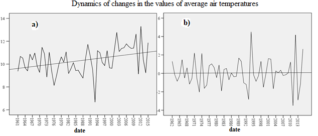
A preliminary examination of the values of the time series showed the absence of missing values and outliers (observation data abnormally far from other values of the time series). Further, the time series is investigated for stationarity. The dynamics of changes in average air temperatures (Fig. 1a) indicates the presence of a trend, and its increase over time, i.e. the original time series is non-stationary.

Figure 1 - Dynamics of changes in the values of average air temperatures with a trend applied: 

a - original series; b - stationary

DOI:10.60797/IRJ.2024.149.129.1

The procedure of taking the first-order difference d=1 transformed the studied series into a stationary ARIMA(p,1,q) (Fig. 1b), resulting in a constant mean around which the series values fluctuate.

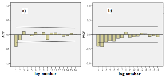
Further, the estimation of the p and q parameters of the model was carried out according to the autocorrelation and partial autocorrelation functions (Fig. 2).

Figure 2 - Autocorrelation ACF(a) and partial autocorrelation PACF(b) functions

DOI:10.60797/IRJ.2024.149.129.2

The order of the moving average MA(q) was determined as the number of significant lags of the autocorrelation function ACF (Fig. 2a). The highest turned out to be the autocorrelation coefficient of the first order MA(1). The order of the autoregressive model AR(p) was chosen from the PACF plot (Fig. 2b), where the lag 2 is distinguished as the last non-zero element, i.e. we have the models AR(1) and AR(2). The choice fell on the candidate models ARIMA(1,1,1) and ARIMA(2,1,1) with and without constants.

The ACF values show a slow decay and the presence of a periodic component in the time series of average air temperatures. The period of the oscillation is equal to the lag at which the correlation coefficient is distinguished. In this case, this is lag 9, but taking into account the first-order difference, we have a 10-year cycle. There is no doubt that this is the result of the manifestation of the 11-year solar activity cycle

The selection of the best of these models was carried out according to:

- BIC information criterion;

- Ljung-Box test for the absence of autocorrelation in the residuals;

- Kolmogorov-Smirnov test for normality of residual distribution.

The normalized Bayesian information criterion BIC

where BICmin – the lowest BIC indicator;

 BICi – indicators of candidate models.

Of the two models, the one with the lower value p is preferred p.

The probability values for all candidate models turned out to be equal to p=0,01.

The significance levels of the Ljung-Box test were very high (p>0,05) for all candidate models (Table 1), therefore, the null hypothesis about the absence of autocorrelation in the residuals can be accepted for all models.

The deviation of the residuals from the normal distribution is considered significant if the significance level of the Kolmogorov-Smirnov test is p<0,05. In the case under consideration, p>0,72, i.e. the residuals do not deviate from the normal distribution.

This indicates that all candidate models are equivalent.

The most popular model selection criteria are the mean absolute percentage error MAPE, which characterizes the accuracy of the forecast, and the coefficient of determination R2, which shows the proportion of the variance explained by the model.

The analysis of the MAPE and R2 values ruled out the models ARIMA(1,1,1) with and without a constant (Table 1).

Thus, at the identification stage, two candidate models ARIMA(2,1,1) with and without a constant remained.

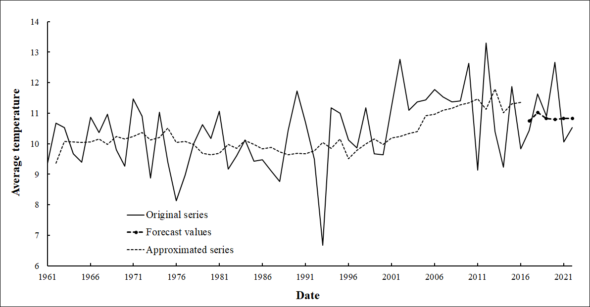
Further selection of an adequate model was based on forecasting the time series values in the retrospective section from 2017 to 2022 (Fig. 3). Figure 3 shows the actual values of the average autumn air temperatures and their forecast values.

Figure 3 - Dynamics of the values of average autumn air temperatures

DOI:10.60797/IRJ.2024.149.129.4

Note: original series (solid curve), approximated series (dashed curve) and forecast values from 2017 to 2022 (dash-dotted)

The absolute errors of the forecast model in the retrospective section – MAPE (Table 2) were calculated according to the actual and forecast values of the studied series.

The model ARIMA(2,1,1) without a constant turned out to be the best, since the mean absolute forecast error for this model was minimal and equal to 5,70; the procedure of taking the first difference of the time series also cancels the model constant.

From the literature, it is known that the MAPE <10% indicates a high accuracy of forecast models.

Analysis of the dynamics of the time series of the values of average air temperatures for the autumn period showed the presence of periodicity caused by the 11-year solar activity cycle.

The average relative forecast error in the retrospective series, which is about 6%, indicates the high accuracy of the proposed model ARIMA(2,1,1).

Analysis of the effectiveness of the selected model showed that the quality criteria for forecasting the values of average autumn atmospheric air temperatures using the proposed model ARIMA(2,1,1) meet all the quality and adequacy criteria required for forecast models.

This indicates that such a complex in nature time series, characterizing the temperature regime of atmospheric air, can be predicted using the Box-Jenkins model.