FRACTAL ANALYSIS OF FINANCIAL MARKETS

Свиридов О.Ю.¹ , Некрасова И.В.²

¹Доктор экономических наук, профессор, ² Кандидат экономических наук, доцент, Южный федеральный университет

ФРАКТАЛЬНЫЙ АНАЛИЗ ФИНАНСОВЫХ РЫНКОВ

Аннотация

В статье ставится под сомнение возможность применения гипотезы эффективного рынка (EMH) для анализа финансовых рынков.

Основная цель данного исследования заключается в анализе методов прогнозирования будущих цен финансовых активов, основанных на концепции фрактальной структуры и долгосрочной памяти финансовых рынков. Фракталы на финансовых рынках интерпретируются либо как инвесторы с различными инвестиционными горизонтами, либо как различные конфигурации движения прошлых цен на графике. В данной статье рассматривается фрактальная структура финансовых рынков, нелинейные методы анализа финансовых рынков, новые подходы к прогнозированию цен финансовых активов, которые позволяют устранить недостатки линейной парадигмы. Результаты исследования, проводимые на валютном рынке и рынке ценных бумаг, подтвердили наличие долгосрочной памяти финансовых рынков.

Ключевые слова: персистентная цена, долгосрочная память, фрактал, принцип самоподобия, Гипотеза эффективного рынка, Гипотеза фрактального рынка.

 

Sviridov O.Y.¹, Nekrasova I.V.²

¹PhD in Economics, Professor, ²PhD in Economics, Associate Professor, Southern Federal University

FRACTAL ANALYSIS OF FINANCIAL MARKETS

Abstract

The article questions the applicability of the Efficient Market Hypothesis (EMH) for analysis of financial markets. The overall goal is to analyze methods of forecasting future prices of financial assets based on the concept of the fractal  structure and long-term memory of financial markets. Fractals in the financial markets are interpreted either as investors with different investment horizons or as a configuration of the price movement on chart. This article examines the fractal structure of financial markets, nonlinear methods of analysis of financial markets, plasticity and long-term memory to long-term investment horizons of financial markets, fractal analysis of financial markets, new approaches to forecast prices of financial assets, which eliminate shortcomings of the linear paradigm. The results of research conducted in the foreign exchange market and securities market, confirmed the existence of long-term memory of the financial markets.

Keywords: price persistence, long-term memory, fraction, the principle of self-similarity, Efficient Market Hypothesis, Fractal Market Hypothesis.

Introduction

Today, the methods for the analysis and prediction of financial market behavior are borrowed from neuroeconomics and have become extremely popular. Many economists believe neuroeconomics as an interdisciplinary field in its broadest sense is a neurobiology of decision-making (decision neuroscience) [1]. It combines neuroscience, economics, psychology, and other disciplines to form the basis of new knowledge about mechanisms of decision-making and helps to simulate the behavior of humans and animals.

An analogue of a neuron in the financial market is a fractal - the price of a financial asset.

Usually it is pointed out that “fractal” came from the Latin “fractus” and close to the English word of fraction or fractional. Therefore, from the mathematic point of view, fractal is a plurality with a fractional (fractal) dimension. The fractal dimension characterizes the way how an object or a time series fills space. In addition, it describes the structure of an object when the zoom factor is changing or while zooming the subject. Under zoom factor escalating is meant. For physical (or geometric) fractals, such conversion occurs in space. The fractal dimension of the time series measures how rugged is the time series itself.

The time series of asset prices is a jagged line. It is not one-dimensional as it is not a direct line; simultaneously, it is not two-dimensional since it does not fill the plane space. Thus, the dimension of a financial range is located between figure one and two. According to expectations, the fractal dimension of a random time series is 1.5.

Fractal is an attractor (a limit and a goal) for the movement of the chaotic system. Why are these notions identical? In a strange attractor as well as in a fractal while increasing it reveals more details (i.e., it triggers the principle of self-similarity). As much as the size of the attractor is changed it is always in the same proportion. The time series is considered fractal when it exhibits a statistical self-similarity; namely, this property is enjoyed by all ranks of financial assets quotations. The self-similarity could be seen during reading ordinary graphs. For instance, it is impossible to distinguish minute, hourly, and daily charts of any product because they are similar and monotonous. In technical analysis, a typical example of a fractal is “Elliott Waves” which construction is also based on the principle of self-similarity.

An additional idea rooted in fractality regards non-integer dimensions which are usually referred to as a one-dimensional, two-dimensional, or three-dimensional integer world. However, there may be a non-integer dimension such as 2.58 (i.e., located between two-axe and three-axe dimensions). Mandelbrot called such dimensions fractals. [2] This idea originates from the opinion that the three-dimensional measurement of the real sphere or cube is inadequate, as soon as in the real world it could be hardly found a perfect sphere or a cube, without scratches or any other inaccurateness. In order to describe complex objects, other measurements should exist. Such measurement of incorrect fractal shapes introduces the concept of a fractal dimension.

From the point of view of classical Euclidean geometry, a crumpled sheet of paper will be a three-dimensional sphere. However, in reality it is still only a two-dimensional sheet of paper even if it is crumpled. Hence, it can be assumed that the new object will have a dimension greater than two but less than three. It hardly fits the Euclidean geometry, but can be well described by fractal geometry which argues that the new object will be located in the fractal dimension equal approximately to 2.5 (i.e., will have a fractal dimension of about 2.5). The physical meaning of this dimension is very simple in that in the classical three-dimensional space, some parts remain empty because of gaps and holes naturally presented in a crumpled sheet of paper.

When applying this theory to the financial markets, we can assume that markets are characterized by various degrees of plasticity defined as the capacity to take and retain form. This definition means that markets can be molded to various degrees in terms of their shapes and functions, and that they are able, to various degrees to retain such changes in their properties even after the molding effort ceases. Thus, plasticity is a dual construct since it requires both fluidity defined as the capacity to take form, and stability defined as the capacity to retain form. All markets are plastic even though their degree of plasticity can change. Therefore, the interplay between fluidity and stability helps us understand market dynamics in more detail.

The term “market plasticity” encapsulates the dynamic and socially constructed nature of markets better than other available terms. Expressions such as ‘‘dynamics”, “development”, and “evolution” lean more toward the process of market change than the characteristics of markets that allows dynamics. Other constructs such as “change” and “fluidity” neglect what is arguably a critical facet of market dynamics, namely its dual character of both fluidity and stability.

There are two important consequences of the plastic character of markets as defined above. First, the ability to retain form allows markets to give form to other entities by, for example, affecting the shape of a particular exchange object, the mode of a specific economic exchange, or the characteristics of an exchange agent. Second, the ability to take form allows markets to host multiple forms simultaneously.

Material and methods

The main method of the fractal time series study is R/S-analysis or the method of rescaled range. It was suggested by the hydrologist Harold Edwin Hurst (1951) who in the mid-20^th century worked at the Nile dam project. [3]

The Hurst exponent can be defined on the interval [0, 1], and is calculated within the following limits:

• 0 ≤ H < 0,5 – data is fractal, the FMH is confirmed, «heavy tails» of distribution, antipersistent series, negative correlation in instruments of value changes, pink noise with frequent changes in direction of price movement, trading in the market is more risky for an individual participant;
• H = 0,5 – data is random, the EMH is confirmed, movement of asset prices is an example of the random Brownian motion (Wiener process), time series are normally distributed, lack of correlation in changes in value of assets (memory of series), white noise of independent random process, traders cannot «beat» the market with any trading strategy;
• 0,5 < H ≤ 1 – data is fractal, the FMH is confirmed, «heavy tails» of distribution, persistent series, positive correlation within changes in the value of assets, black noise, the trend is present in the market.

The Hurst index could be also used as a measure of volatility of the data series. Peters (1994) highlights in his «Fractal Market Analysis: Applying Chaos Theory to Investment and Economics» that in the analysis of stock risks it is preferable to use the fractal dimension instead of the standard deviation. [4] The standard deviation is good while it characterizes variability of random series. If to deal with market as a stochastic process, in this case the use of standard deviation as the main characteristics of risk values is justifiable enough. If to admit that market is not stochastic, but chaotic, fractal dimension as a measure of non-linearity of price movements is much better suited.

Why does an effect of the price inertia in relation to the previous motion appear in the financial markets? This fact can be explained based on the psychology of human memory. The Hurst index of over 0.50 also confirms the presence of non-volatile memory market – the present depends on the past and the future depends on the present.

Those who calculate the Hurst index, based on market prices, often stand the arising question of what ranks to explore – data series or data changes. For instance, it could be the logarithm of the current value to the previous one which is usually used in the analysis of market quotations. Analysis has shown that the normalized logarithmic scale of random series of changes is much smaller than the scale of the normalized logarithmic linear (rising or falling) series changes. As the result, the Hurst index calculated on the logarithms of linear series changes reach huge quantities.

Therefore, if we take a series of data that evince some signs of trending, calculate logarithms changes on it, the Hurst exponent of such series will be well above 1. That is why it will be used the classic model of the Hurst index calculation according to the initial data series. [5]

Results

We have chosen interval of one year and made calculation for the currency pair EUR/USD. The interval is equal to 1 week, the number of observations – 52. The data used for this calculation was retrieved at the FOREX - FXTMPIRE // http://ru.fxempire.com/currencies/eur-usd/tools/historical-data/ . [6]

The results of our calculations are shown in Table 1.

Table 1 – Hurst exponent calculation results on the closing prices of the currency pair EUR/USD (N=52) for the 2015 year

Date	Close price	(xi  - X)	Ʃ(xi - X)
27 December 15	1,09695	-0,0121	-0,012120577
20 December 15	1,08697	-0,0221	-0,034221154
13 December 15	1,09808	-0,0110	-0,045211731
6 December 15	1,08813	-0,0209	-0,066152308
29 November 15	1,05832	-0,0508	-0,116902885
22 November 15	1,06375	-0,0453	-0,162223462
15 November  15	1,07004	-0,0390	-0,201254038
8 November  15	1,07295	-0,0361	-0,237374615
1 November  15	1,10229	-0,0068	-0,244155192
25 October 15	1,10048	-0,0086	-0,252745769
18 October 15	1,13582	0,0267	-0,225996346
11 October 15	1,13685	0,0278	-0,198216923
4 October 15	1,12195	0,0129	-0,1853375
27 September 15	1,1202	0,0111	-0,174208077
20 September 15	1,129	0,0199	-0,154278654
13 September 15	1,13423	0,0252	-0,129119231
6 September 15	1,11544	0,0064	-0,122749808
30 August  15	1,12114	0,0121	-0,110680385
23 August 15	1,1378	0,0287	-0,081950962
16 August 15	1,1094	0,0003	-0,081621538
9 August  15	1,09583	-0,0132	-0,094862115
2 August 15	1,09677	-0,0123	-0,107162692
26 July 15	1,0974	-0,0117	-0,118833269
19 July 15	1,083	-0,0261	-0,144903846
12 July 15	1,11295	0,0039	-0,141024423
5 July 15	1,09949	-0,0096	-0,150605
28 June 15	1,09749	-0,0116	-0,162185577
21 June 15	1,13616	0,0271	-0,135096154
14 June 15	1,12245	0,0134	-0,121716731
7 June 15	1,11025	0,0012	-0,120537308
31 May 15	1,09565	-0,0134	-0,133957885
24 May 15	1,09913	-0,0099	-0,143898462
17 May 15	1,1446	0,0355	-0,108369038
10 May 15	1,11955	0,0105	-0,097889615
3 May 15	1,1187	0,0096	-0,088260192
26 April 15	1,08658	-0,0225	-0,110750769
19 April 15	1,08085	-0,0282	-0,138971346
12 April 15	1,06066	-0,0484	-0,187381923
5 April 15	1,09949	-0,0096	-0,1969625
29  March 15	1,08827	-0,0208	-0,217763077
22 March 15	1,08253	-0,0265	-0,244303654
15 March 15	1,04839	-0,0607	-0,304984231
8 March 15	1,08448	-0,0246	-0,329574808
1 March 15	1,1161	0,0070	-0,322545385
22 February 15	1,13805	0,0290	-0,293565962
15 February 15	1,13977	0,0307	-0,262866538
8 February 15	1,13137	0,0223	-0,240567115
1 February 15	1,13073	0,0217	-0,218907692
25 January 15	1,11423	0,0052	-0,213748269
18 January 15	1,15613	0,0471	-0,166688846
11 January 15	1,18418	0,0751	-0,091579423
4 January 15	1,20065	0,0916	2,68674E-14
Arithmetic mean Х	1,109070577	Maximum	2,68674E-14
Standard deviation S	0,0297	Minimum	-0,3296
Scope R	(2,68674E-14)-(-0,329574808)=		0,3296
Normalized scope R/S	0,3296/0,0297=		11,1123
Log(R/S)	Log(11,1123) =		1,0458
Log(N*π/2)	Log(52*3,1416/2) =		1,9121
Hurst index Н	1,0458/1,9121=		0,5469
Calculation R/ST	11,1123*0,998752+1,051037 =		12,1494
Log(R/SТ)	Log(12,1494) =		1,0846
Hurst-Naiman index НТ	1,0846/1,9121*(-0,0011*Ln(52)+1,0136) =		0,5738

The calculation results show that the market has a memory on a time interval of one year, since H = 0.5469.

Next, we have chosen the different currency pair GBP / USD, the same number of observations (N = 52), the interval - 1 week. The calculation results are presented in Table 2.

Table 2 – Hurst exponent calculation results on the closing prices of the currency pair GBP/USD (N=52) for the 2015 year

Date	Close price	(xi  - X)	Ʃ(xi - X)
27 December 15	1,4733	-0,0536	-0,053615192
20 December 15	1,49254	-0,0344	-0,087990385
13 December 15	1,4893	-0,0376	-0,125605577
6 December 15	1,52278	-0,0041	-0,129740769
29 November 15	1,51033	-0,0166	-0,146325962
22 November 15	1,50304	-0,0239	-0,170201154
15 November  15	1,51873	-0,0082	-0,178386346
8 November  15	1,52345	-0,0035	-0,181851538
1 November  15	1,50471	-0,0222	-0,204056731
25 October 15	1,54271	0,0158	-0,188261923
18 October 15	1,53077	0,0039	-0,184407115
11 October 15	1,54361	0,0167	-0,167712308
4 October 15	1,5305	0,0036	-0,1641275
27 September 15	1,51738	-0,0095	-0,173662692
20 September 15	1,51863	-0,0083	-0,181947885
13 September 15	1,55227	0,0254	-0,156593077
6 September 15	1,54229	0,0154	-0,141218269
30 August  15	1,51694	-0,0100	-0,151193462
23 August 15	1,53967	0,0128	-0,138438654
16 August 15	1,56896	0,0420	-0,096393846
9 August  15	1,5649	0,0380	-0,058409038
2 August 15	1,54915	0,0222	-0,036174231
26 July 15	1,56216	0,0352	-0,000929423
19 July 15	1,55107	0,0242	0,023225385
12 July 15	1,56055	0,0336	0,056860192
5 July 15	1,55131	0,0244	0,081255
28 June 15	1,55663	0,0297	0,110969808
21 June 15	1,57451	0,0476	0,158564615
14 June 15	1,5876	0,0607	0,219249423
7 June 15	1,55536	0,0284	0,247694231
31 May 15	1,52712	0,0002	0,247899038
24 May 15	1,52837	0,0015	0,249353846
17 May 15	1,54957	0,0227	0,272008654
10 May 15	1,57271	0,0458	0,317803462
3 May 15	1,54432	0,0174	0,335208269
26 April 15	1,51478	-0,0121	0,323073077
19 April 15	1,5186	-0,0083	0,314757885
12 April 15	1,49556	-0,0314	0,283402692
5 April 15	1,4631	-0,0638	0,2195875
29  March 15	1,49154	-0,0354	0,184212308
22 March 15	1,48695	-0,0400	0,144247115
15 March 15	1,49433	-0,0326	0,111661923
8 March 15	1,47384	-0,0531	0,058586731
1 March 15	1,50311	-0,0238	0,034781538
22 February 15	1,54282	0,0159	0,050686346
15 February 15	1,53886	0,0119	0,062631154
8 February 15	1,53928	0,0124	0,074995962
1 February 15	1,52385	-0,0031	0,071930769
25 January 15	1,50546	-0,0215	0,050475577
18 January 15	1,49882	-0,0281	0,022380385
11 January 15	1,51552	-0,0114	0,010985192
4 January 15	1,51593	-0,0110	1,46549E-14
Arithmetic mean Х	1,526915192	Maximum	0,3352
Standard deviation S	0,0284	Minimum	-0,2041
Scope R	0,3352 -(-0,2041)=		0,5393
Normalized scope R/S	0,5393/0,0284=		18,9734
Log(R/S)	Log(18,9734) =		1,2781
Log(N*π/2)	Log(52*3,1416/2) =		1,9121
Hurst index Н	1,2781/1,9121=		0,6684
Calculation R/ST	18,9734*0,998752+1,051037 =		20,0007
Log(R/SТ)	Log(20,0007) =		1,3010
Hurst-Naiman index НТ	1,3010/1,9121*(-0,0011*Ln(52)+1,0136) =		0,6884

The study results also confirm the existence of long-term memory of the financial markets, as Hurst exponent is 0.6684.

Then a computer program «Meta Trader 4" was used to obtain more reliable data on the presence of long-term memory of the financial markets. «Meta Trader 4» is a platform for trading Forex, analyzing financial markets and using Expert Advisors.

Next on the programming language MQL4, the company MetaQuotes Software Corp., indicator has been written on the basis of the Hurst formula. Indicator defines the value of H for each day bar, based on historical data and a predetermined constant period - N and constant - .

The observations were made from the end of 2007 to July 2016 for the two currency pairs EUR / USD and GBP / USD (Figures 1, 2). The closing price of the daily bars were taken as the data, the number of observations was 3000 ( N = 3000) for each currency pair (the period from 11. 2007 year to 07. 2016 year.), constant .

The study showed that under a large sample (N = 3000) the dynamics of the indicator curve has fairly smooth structure. The minimum value of the Hurst index did not fall below 0.8073 for the EUR / USD and 0.8441 for the pair GBP / USD during the given period. The maximum value of the Hurst exponent for the EUR / USD pair was 0.847, and for the pair GBP / USD is slightly higher - 0.8505. This indicates the presence of long-term memory of the currency markets.

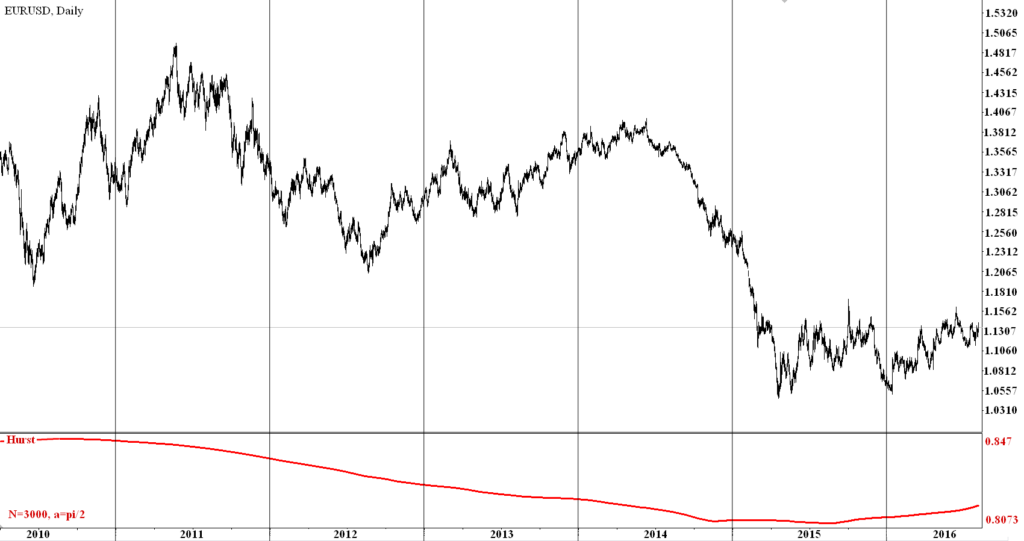
Figure 1 – The dynamics of daily bars of the currency pair EUR / USD and the values of the Hurst exponent on the time interval from 03.2010 to 07. 2016.

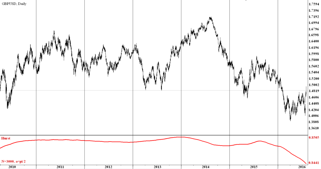
Figure 2 – The dynamics of daily bars of the currency pair GBP/USD and the values of the Hurst exponent on the time interval from 03.2010 to 07. 2016.

Similar results indicator shows for the stock market. The observations were made for the five indices: two Russian - RTS, MICEX (MCX) and three foreign indexes - NasDaq, DowJones, SnP500. (Figures 3, 4). The closing price of the daily indices bars were taken as the data, the number of observations was 1000 (N = 1000) for each index (the period from 07. 2013 year to 07. 2016 year.).

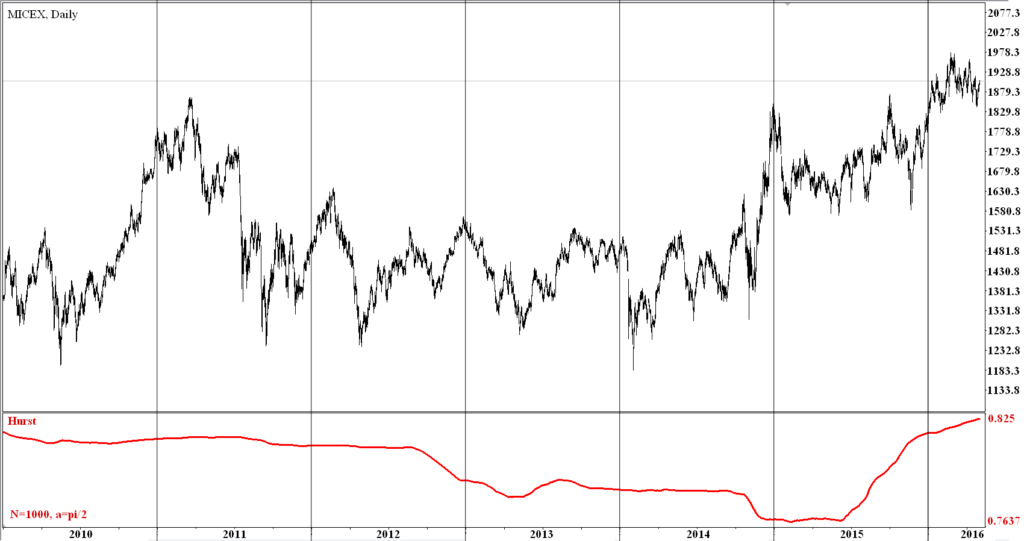
Figure 3 – The dynamics of daily bars of the MICEX Index and the values of the Hurst exponent on the time interval from 12. 2009 – 07. 2016.

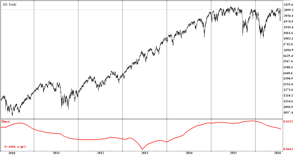
Figure 4 – The dynamics of daily bars of the SnP500 Index and the values of the Hurst exponent on the time interval from 12. 2009 – 07. 2016.

Studies have shown that the values of the Hurst exponent for all indices ranged from 0.83 to 0.76. Russian indices values below for a few hundredths of a unit compared with foreign indices.

Thus, our calculations show that market events and economic indicators are not random. This conclusion was reached for all the calculated data series at different time intervals. The market is inert and has a memory. Moreover, the longer the interval, the more pronounced the market memory. This confirms the validity of the FMH which is seen as an alternative to the EMH. Since the Hurst index can be helpful for calculating fractal dimension, it is considered a necessary element of the FMH.

Conclusion

The results of our calculations demonstrate that market events and economic indicators are not random phenomena. The market has a fractal structure and a long-term memory and plasticity. This conclusion has been reached for all data series in different time intervals. Therefore, the FMH can be applied successfully to economic phenomena. The assumption that investment decisions can be predicted based on the analysis of neural mechanisms of the information influence on fractals will allow to open new horizons in understanding of the investor behavior in financial markets. In order to understand the process of investment decision-making, the following scheme could be recommended:

1. On the first step, the formulation of a problem creates a view about the purpose and context of the decision. It integrates information about the internal conditions of the organism and environmental factors, such as famine or level of threat in the context of future action.
2. The next step is determined by the value or valuation of the choosing procedure with particular behavioral alternatives.
3. On the third step, alternative solutions are compared and the best solution is selected. This step is called action selection.
4. After implementation of a selected action the results are calculated and efficiency is evaluated.
5. The last step is training. Training means updating information stored in the memory, so that all subsequent steps would be implemented with greater efficiency.

Список литературы / References

1. Klucharev V. A., Smidts A., Shestakova A.N. Neuroeconomics. The Neurobiology of Decision-making. // Experimental Psychology. – 2011. – Vol.4, № 2. – P. 14–35.
2. Mandelbrot B. B., J. W. van Ness. “Fractional Brownian Motion, Fractional Noises and Application” // SIAM Review, 10, 1968. – P. 422–37.
3. Hurst H.E. “Long-term storage of reservoirs: an experimental study” // Transactions of the American Society of Civil Engineers. – 1951. – Vol. 116. – P. 770-799.
4. Peters Edgar E. Fractal Market Analysis: Applying Chaos Theory to Investment and Economics. New York: John Wiley and Sons, 1994.
5. Некрасова И.В. Показатель Херста как мера фрактальной структуры и долгосрочной памяти финансовых рынков // Международный научно-исследовательский журнал. – 2015. №7-3 (38). – С. 87-91.
6. Official site FOREX – FXTMPIRE [Electronic resource]. – URL: http://ru.fxempire. com/currencies/eur-usd/tools/historical-data/ (Accessed 12.10.2016)

 Список литературы латинскими символами / References in Roman script

1. Klucharev V. A., Smidts A., Shestakova A.N. Neuroeconomics. The Neurobiology of Decision-making. // Experimental Psychology. – 2011. – Vol.4, № 2. – P. 14–35.
2. Mandelbrot B. B., J. W. van Ness. “Fractional Brownian Motion, Fractional Noises and Application” // SIAM Review, 10, 1968. – P. 422–37.
3. Hurst H.E. “Long-term storage of reservoirs: an experimental study” // Transactions of the American Society of Civil Engineers. – 1951. – Vol. 116. – P. 770-799.
4. Peters Edgar E. Fractal Market Analysis: Applying Chaos Theory to Investment and Economics. New York: John Wiley and Sons, 1994.
5. Nekrasova I.V. Pokazatel’ Hursta kak mera fraktal’noj structury i dolgosrochnoj pamyati finansovych rynkov [The Hurst index as a measure for the fractal structure and long-term memory of financial markets] // Mejdunarodnyj nauchno-issledovatel’skij jurnal [International Research Journal] – 2015. – №7-3 (38). – P. 87-91. [in Russian]
6. Official site FOREX – FXTMPIRE [Electronic resource]. – URL: http://ru.fxempire. com/currencies/eur-usd/tools/historical-data/ (Accessed 12.10.2016)