Оптимизация траектория космического аппарата с помощью идеально-регулируемого двигателя в окрестности круговой орбиты

Currently, the problems of optimizing the trajectories of spacecraft (SC) are one of the main areas of research in the field of celestial navigation and space mission planning. The problem of trajectory optimization is of particular interest of optimizing the trajectory for spacecraft with an ideally controlled engine capable of providing two and three channel control, especially in the vicinity of a circular orbit. Such systems require a systematic approach to planning and controlling maneuvers to achieve specified orbital parameters or perform a specific space mission. One important aspect of such planning is taking into account resource constraints and ensuring efficient use of fuel during maneuvers.

In the 60s, the use of electric rocket engines (ERE) in spacecraft began. Due to their high specific impulse, ERE can significantly reduce fuel consumption for orbital maneuvering. Despite the low thrust characteristic of ERE compared to traditional liquid rocket engines, their long-term operation has become possible. Electric propulsion with Low-thrust has been successfully used in various interplanetary missions. For an idealized mathematical model of electric propulsion, a model of an ideally regulated (IR) engine is used. Within the framework of this model, the reactive power of the IR engine is considered constant, although the thrust and exhaust velocity can vary arbitrarily

Optimal control of the relative motion of SC near circular orbits is crucial for various space missions, including rendezvous and docking, formation missions, deployment and maintenance of low-orbit systems for communications and Earth sensing, and missions between close orbits. Determining the appropriate control strategy is vital to ensure the transfer of the system from the initial state to the final state with minimal fuel consumption, which is essential for economic efficiency and the successful execution of space missions.

Minimizing fuel consumption is equivalent to minimizing a specific functional. To achieve this objective, various methods are employed, including those based on Pontryagin's maximum principle

The paper discusses the optimization problem of a trajectory with limited thrust for an ideally controlled engine using a method based on the Pontryagin maximum principle, which involves considering derivatives of a certain function. Solutions to this problem serve as initial approximations for numerically optimizing a trajectory with constant exhaust velocity and limited thrust

The purpose of this paper is to optimize the control of spacecraft relative motion using an ideally regulated engine near a circular orbit to minimize overall fuel consumption. The author conducts a detailed analysis of two and three-channel control and proposes optimization methods to achieve optimal results under limited resource conditions. Additionally, the author examines the closed-form IR trajectory optimization problem with limited thrust for both two- and three-channel control. The closed-form solution to this problem serves as initial assumption values for the numerical optimization of a constant-velocity trajectory with limited exhaust velocity

The study of such problems is crucial for improving navigation technologies and enhancing the efficiency of space missions within limited resources and time constraints. For instance, the use of two-channel control is often necessitated by the limited capabilities of the control system, the need to ensure radio communication conditions or mutual visibility of approaching spacecraft, and various other factors.

To analyze the relative motion of SC near circular orbits, the development of special mathematical models of motion is required. One of the most common mathematical models of relative motion in the vicinity of circular orbits is the Hill-Clohessy-Wiltshire (HCW) model

2.1. Formulation of the problem

There are known initial and final phase vectors of the relative motion of a SC with an ideally regulated engine in the vicinity of a given circular orbit: . It is assumed that the SC moves in a central gravitational field, where it is affected only by the main term of gravitational acceleration and reactive acceleration. It is necessary to define the state trajectory as a piecewise continuous function of time  Each state trajectory is implicitly generated by the control (reactive acceleration program) , according to the system dynamics . Thus, the problem is to determine the control that ensures the transfer of the dynamic system under consideration from a given initial state to a given final state in a fixed time interval with minimal fuel consumption

2.2. Optimizing the control of an ideally regulated engine

Let us consider the motion of the SC relative to point O, which moves around the Earth in an unperturbed circular orbit with a certain radius r0. For convenience, we introduce a coordinate system where the x axis coincides with the direction of the radius vector of point O, the y axis is in the transversal direction, and the z axis complements the coordinate system to the right. In this coordinate system, the HCW equations in dimensionless variables take the following form: 

(1)

where t – time; x, y, z – spacecraft coordinates; vx, vy, vz – components of the spacecraft velocity vector; ax, ay, az – components of the reactive acceleration vector.

It is required to transfer system (1) from a given initial position to t = 0:

(2)

to the final position specified at a fixed time :

(3)

with minimal fuel consumption.

2.3. Minimizing fuel mass

The problem of minimizing the fuel mass is equivalent to the problem of minimizing the functional

(4)

where  - magnitude of reactive acceleration.

Separation into two independent subproblems becomes possible for the motion of the spacecraft: in the orbital plane and along the z axis. Thus, motion in the orbital plane and outside it can be described by a system of differential equations:

(5)

With functionals 

(6)

where 

Boundary conditions, taking into account (2), (3), can be written as:

(7)

We can write the Pontryagin function for both subproblems as: 

(8)

where the vector p represents the conjugate variables. According to the maximum principle, the optimal control is determined by maximizing the Hamiltonian with respect to the control variable a. Thus, we obtain an expression for optimal control in the following form:

(9)

we substitute (9) into (8) and obtain the Hamiltonian 

(10)

The system of differential equations describing the optimal motion and corresponding to the Hamiltonian (10) takes the following form:

(11)

The solution to system (11) has the form:

(12)

(13)

(14)

where Ф(t) – fundamental matrix of a homogeneous system  – the initial value of the vector of conjugate variables for motion in the plane of the reference orbit, at t = 0.

To solve the optimal control problem, it is necessary to determine the value of p0 at which the boundary conditions (7a) and (7b) are satisfied. It is clear that from (13) the optimal solution can be derived in the following form:

(15)

where p0z is the initial value of the vector of conjugate variables for motion along the normal to the plane of the reference orbit, at t = 0.

Matrices Ф and Г are calculated analytically, also introducing the notation c = cost, s = sint, we obtain:

for three-channel control and,

for two-channel control,

After determining the initial vector of conjugate variables according to formulas (15), the optimal trajectory is calculated using expression (13), and the optimal control is determined using expression (12) and expression (15). The total characteristic velocity and total costs are then determined.

Let us consider the motion of the spacecraft relative to point O, moving in an undisturbed near-Earth circular orbit with a radius of 6871 km. Let us take the gravitational parameter of the Earth equal to 3.9860044*1014 m3/s2. Let us consider the problem of flying in  =14400 s from a point in phase space r0  = (10,100,-5)т  km,  v0  = (-1,10,3)т  m/s to the origin of coordinates, that is to point rf = 0 km, with velocity vf = 0 m/s. In this case, the initial mass of the spacecraft is 1000 kg, and the specific impulse of the propulsion system is 220 s.

Figure 1 shows the optimal IR trajectory for the case of three- and two-channel control, as well as the dependence on the time of reactive acceleration for three- and two-channel control, on which the starting and ending points (meeting points) are marked after performing several maneuvers. The optimality of this trajectory is due to the fact that it ensures effective achievement of the goal with minimal fuel consumption. The starting and ending points on the trajectory indicate the location of the SC before and after performing maneuvers, and the meeting point represents the moment when the vehicles approach each other. It is important to note that carrying out several maneuvers during the movement allows you to optimize the trajectory and achieve the desired position in outer space.

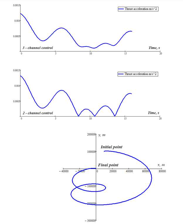
Figure 1 - Optimal IR trajectory and time dependence of reactive acceleration for three and two-channel control

DOI:10.60797/IRJ.2024.144.24.1

Table 1 shows the results of calculating the components of velocity impulses in the time range from 0 to 15.963 (in dimensionless variables, you need to multiply by scaleT = 902.113s) for two and three-channel control. The first column represents time (t), and the next three columns represent the components of velocity change (projection) along the three axes: X, Y, and Z, respectively.

Note that time and velocity impulse components are represented in dimensionless variables. To enter a specific unit of measurement, you need to multiply them by “scaleT = 902.113s”, and by “scaleV = V0”, where V0 is the velocity of movement in a circular orbit.

Table 2 shows the results of calculating the magnitudes of velocity impulses and fuel consumption in the time range from 0 to 15.963 (in dimensionless variables). These data make it possible to evaluate the necessary maneuvers to achieve the required trajectory using fuel.

From Table 2, it is evident that, based on the required fuel consumption, two-channel control proves to be highly efficient and nearly indistinguishable from three-channel control. Notably, for two-channel control, at time t=0 s, the maneuver is 10.488 m/s with a fuel consumption of 4.848 kg, at t = 14400 s, the rendezvous maneuver reduces to 0.0027 m/s, resulting in minimal fuel consumption of only 0.00125 kg. On the other hand, for three-channel control, at t = 0 s, the maneuver is 10.488 m/s with a fuel consumption of 4.848 kg, at t=14400 s, the rendezvous maneuver decreases to 0.0024 m/s, and the fuel consumption reaches a minimal value of only 0.00111 kg.

To validate the obtained analytical solution, the analytical trajectory optimization results were compared with those obtained through numerical solution of the corresponding boundary value problem using the maximum principle. For the numerical solution, a continuous continuation method with respect to a parameter was employed, similar to the approach proposed in

Figure 2 shows isolines, that is, the dependence of the functional on the time of the start of the maneuver (engine start) and the duration of the maneuver for the cases of two and three-channel control.

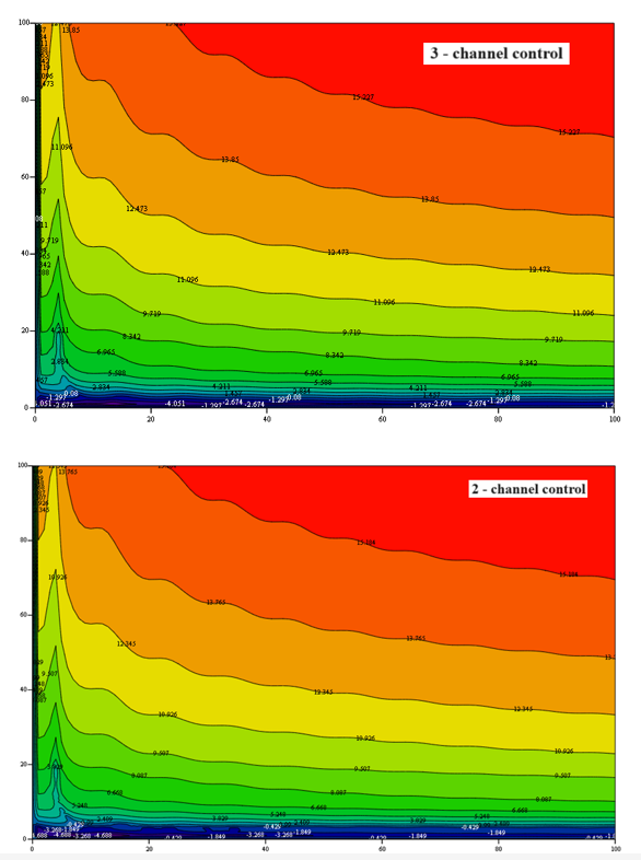
Figure 2 - Dependences of the functionality on the start time of the maneuver and the duration of the maneuver for the cases of two and three-channel control

DOI:10.60797/IRJ.2024.144.24.4

Figure 2 shows zones with the same functional values, that is, the time the engine is turned on and the duration of these maneuvers. The presented contour lines show the dependence of the function on the start time of the maneuver (engine start) and the duration of the maneuver, providing an overview of how the function changes depending on the duration of the maneuver. They help identify areas with similar fuel consumption, as well as areas with high and low fuel consumption according to functional values. This will lead to the fact that with two-channel control, the minimum fuel consumption in accordance with the isoline graph will be in the range from -0.429 to 4.423, which corresponds to the dark blue region where the minimum functional values are achieved. When the engine runs almost continuously, three-channel control can reduce fuel costs by almost 5% compared to two-channel control. Thus, from the perspective of required fuel consumption, two-channel control becomes practically indistinguishable from three-channel control when maneuvering above 2 mm/s.

The paper considers the problem of optimizing the trajectory of a spacecraft using an ideally regulated engine in the vicinity of a circular orbit. The problem of flying to a given point, velocity and fixed time is considered. Statements of the optimal control problem for the cases of two and three-channel control are presented. With two-channel control, there is a limitation on the direction of the thrust vector, and the radial component of the thrust is zero. The problems of minimizing fuel consumption for the limited power of a spacecraft propulsion system are considered. For this problem, an analytical solution was obtained in explicit form, which can be used as an initial approximation for solving many practical problems. When the engine runs almost continuously, three-channel control can reduce fuel costs by almost 5% compared to two-channel control. Thus, from the perspective of required fuel consumption, two-channel control becomes practically indistinguishable from three-channel control when maneuvering above 2 mm/s. Optimal control with two-channel control turns out to be extremely important due to its frequent use due to control system limitations, the need to ensure radio communication or mutual visibility of approaching spacecraft, and other factors.