ПОСЛЕДСТВИЯ ФИНАНСОВОГО КРИЗИСА В ЛИТВЕ, АВСТРИИ И КАЗАХСТАНЕ

Конахбаев Е.Б.

Магистр экономических наук, Вильнюсский Университет

ПОСЛЕДСТВИЯ ФИНАНСОВОГО КРИЗИСА В ЛИТВЕ, АВСТРИИ И КАЗАХСТАНЕ

Аннотация

Исследование направлено на выявление соответствующего метода для практического определения последствий финансового кризиса в Литве, Австрии и Казахстане. В частности, в работе использованы фиктивная переменная (линейная модель вероятности), нелинейная экспоненциальная модель, обобщенная модель авторегрессионной условной гетероскедастичности (GARCH), модели Логит-Пробит, параметрическая квантильно-регрессивная модель и модель с полиномиальными распределенными лагами (авторегрессивная модель, динамическая модель) для анализа сходств и различий последствий финансовых кризисов в наблюдаемых странах. На основе анализа теории и эмпирических исследований, автором было выбрано шесть переменных для анализа со статистическими данными за период 15 лет (с первого квартала 2000 года по четвертый квартал 2014 года): Потребительские цены, Государственные расходы, процентная ставка, обменный курс, Импорт и экспорт. Данные были собраны из базы Евро-Стат и статистических данных центрального банка Республики Казахстан, измеряются в миллионах евро.

Ключевые слова: финансовый кризис, последствия, Литва, Австрия, Казахстан.

 

Konakhbayev Ye.B.

Master of Economic Sciences. Vilnius University.

THE IMPACT OF FINANCIAL CRISIS IN LITHUANIA, AUSTRIA AND KAZAKHSTAN 

Abstract

The research intends to utilize an appropriate method to provide empirically the impact of financial crises in Lithuania, Austria and Kazakhstan. In particular the study intends to use dummy variable (linear probability model), non-Linear exponential model, Generalized autoregressive conditional heteroskedasticity model (GARCH), Lobit-Probit models, a parametric Quantile regression model and Polynomial distributed lags model to analyse similarities and different consequences of the financial crises in observed countries. Based on the theory and analysis of empirical studies the author selected six variables into research for 15 years periods (from quarter one of 2000 to quarter four of 2014): Consumer price, Government Expenditure, Interest rate, Exchange rate, Import and Export. The data are sourced from Euro-Stat data base and Kazakhstan central bank statistics, measured in million of Euros.

Keywords: financial crisis, impact, lithuania, kazakhstan, austria.

The financial and economic crises, fortunately, does not happen every day. However, the significance of such relatively "rare" events is extremely high. The massive destruction of market participants, sometimes the biggest, strongest market disruption, developing into an economic depression, lost jobs and years, frustration and values are not a complete list of tragedies that bring the crisis to millions of people. Events of such magnitude, their causes in the past and the future, quite naturally, attracted the most attention of scientific, not only scientific public.

The powerful shock of financial and real markets appeared the credit crisis (credit crunch) in 2007-2009. Having undergone a turn of the century under the influence of asset securitization qualitative change, the global financial system collapsed in 2008 "vaporizing" the value of total financial assets of about 15 trillion dollars (IMF, 2012). If the ratio of financial assets to world GDP in 2007 reached 421 percent, while by 2011 it decreased to 352 percent. Compression, up to certain limits, a bloated financial system - a phenomenon generally positive, but its catastrophic reduction is highly undesirable because of the disorganization of the entire economy, including the real markets. Minimizing losses, of course, depends on the accuracy of prediction of the onset of the next financial crisis. However, as often happens, the formulation of the problem is much easier to answer to it.

The crisis in 2007-2009 found gaping holes in our knowledge of the structure and behavior of the financial system, its interaction with the economy as a whole. Meanwhile, the "surprise" the grand catastrophe that has matured over the years as it is not sad to admit, largely due to the lack of scientific methodology and models on which to learn, play and predict the effects of such an order of complexity. There was a paradoxical situation. Crises for centuries accompanied the economic life, attracted the attention of prominent minds, they devoted an enormous literature, and long-term studies. Despite this, our knowledge of the phenomenon, the scale of the devastation is much superior to natural disasters, remain incomplete and limited. The complex and multidimensional phenomenon - the financial crisis - is not an operational concept. Information about it is largely descriptive in nature, structured enough, inconsistent, fragmented and sometimes deliberately distorted. By virtue of "rarity" of the crisis their statistics are short and unreliable. These difficulties necessarily arise even when using specific quantifiable approximation of crisis, such as the imbalance between aggregate savings and investment.

Now, with the influence of leading economists, including G. Stiglitz, P. Krugman, G. Akerlof, R. Schiller and many others there is actively developed a "new economic paradigm" - the scientific concept that actualizes the idea of G. Keynes, I. Fisher and H. Minsky on financial bubbles and crises [14]. It aims to explain the conditions of such extreme events and form the scientific basis for practical recommendations in terms of minimizing the negative effects on the economy [17]. The methodology of solving such problems - it is the theory of complex systems, since the behavior of financial markets, where "everything depends on everything", generally corresponds to the behavior of objects such complexity [18]. However, specification of the principles and provisions of the theory in relation to the financial markets is very difficult process of accumulation of knowledge about their functioning.

This process is greatly complicated by the extremely high information requirements to the object of study. So-called "high-frequency" arrays financial information is already measured in multiples of 109, and it is - is not the limit. Huge amount of information reflects qualitatively new features of modern financial systems. For instance, the studies of "Econophysics" show in the vicinity of the critical state (the crisis), the probability distribution of financial variables do not have the characteristic scale and are not Gaussian, but the degree, especially in their "tails" [20]. In such systems, the distribution of the laws of crises (the critical states of the system) is significantly different from the distribution of defaults in the portfolio of a typical investor. This, in particular, explains why it is so difficult to obtain conclusive generalization of well-designed macro-copulative models formalize the loss of investors, depending on the correlation of defaults of assets [21].

Analysis of the state of microfinance was in full accordance with the policy of extremely low interest rates of refinancing, following the credit crisis. On the one hand, the standard models, such as IS-LM, designed for "normal" markets were not able to predict and adequately explain the conditions for the occurrence of large shocks. Following their recommendations in many ways, the central banks almost to the limit lowered the refinancing rate, but, nevertheless, the balance of supply and demand in key markets has not been restored. As a result, not only the money market was trapped, but, as the experience of the leading world economies, aggregate savings continue to significantly exceed the amount of investment [15]. Analytically, these processes have transformed the LM curve in the trivial identity and curve IS - equilibrium on real markets - the "disappeared", and here to stay. As a result, the analytical tools used by central banks in need of radical modernization in order to contribute to the success of the "unorthodox" monetary policy in the post-crisis period.

The objective difficulties in the study of modern financial systems is one of the reasons for the use of simple models (example is the work of T. Adrian and H. Shin, D. Farmer, as well as a number of other researchers, including the author) [22-24]. Such models, focusing on system-wide property market (and crises), are not only effective, but also, in many cases, do not have alternatives. The use of simple models seems justified to create integrated systems for macro-financial and macro-economic models, especially in studies of inertial and low-frequency processes.

In the absence of information on the properties of the true distribution of the states of simple models do not increase the errors caused by the fragmentation of knowledge about the behavior of the markets under uncertainty. In light of the fact that the development of a comprehensive model of the crisis, as a special socio-economic phenomenon, forms the subject of independent and long-term studies, it seems reasonable to supplement simple way of forecasting events of this class of complexity.

For example, the proposed model, simplifying the complex and poorly understood phenomena in the financial crisis, only requires the ability to recognize situations of crisis or lack thereof. The sequence of random variables corresponding indicator allows, as will be shown below, calculate the probability of a crisis for the simple hypotheses of their distributions. In addition, the model determines not a crisis, and so-called "critical situation", which may be the world financial system. By this is meant for the solution of equal probability of "survival" and "collapse" of the financial system. Of course, a 50-percent chance of a priori identical onset of the crisis, but this threshold is probably the easiest way indicates a qualitative change in the development of the financial system.

This research intends to utilize an appropriate method to provide empirically the impact of financial crises in Lithuania, Austria and Kazakhstan. In particular the study intends to use dummy variable (linear probability model), non-Linear exponential model, Generalized autoregressive conditional heteroskedasticity model (GARCH), Lobit-Probit models, a parametric Quantile regression model and Polynomial distributed lags model to analyse similarities and different consequences of the financial crises in observed countries.

Based on the theory and analysis of empirical studies the author selected six variables to determine the impact of financial crises in Lithuania, Kazakhstan and Austria for 15 years periods (quarter one of 2000 to quarter four of 2014). The independent variables are Consumer price, Government spending, Interest rate, Exchange rate, Import and Export while financial crisis is dependent variable. The data are sourced from Euro-Stat data base and Kazakhstan central bank statistics, measured in million of Euros.

 

 

Research Methodology

Definition of Variable:

• Exchange rate is measured as ratio of a foreign currency (Euro) to national currencies;
• Interest rate is represented by short term treasury bill rates;
• Consumer price is measured by Consumer price Index of observed countries in Euros;
• Government spending is measured in terms of thousand EUR per capita and as a percentage of GDP.
• Import is the importation of all the goods and services to the rest of the world;
• Export is exportation of all the gross goods and services over the border of national country;
• Crisis is unobserved variable and the outcome of all the independent variables.

Equations used to assess Prediction of Financial Crises:

• Non-Linear Y_t= αe^bxt +ε_t
• Distributed Lags     Y_t = C₀X_t+C₁X_t+C₂X_t+ε_{t   ............} {Y_t= (Ʃ_i=C_iL_i)X_t+ε_t}
• GARCH Û_t = β₀ + β₁ȳ² + β₁ȳ³ + β₁ȳ⁴  ..... σ² = α₀ +Û²_{t-1 +} σ²_t
• Probit and Lobit Y_t = 1/1+e ^-(β0+β₁^X_t⁾
• Quantile ϛ_p (x_t) = q(x_t,ᴓ) ....... = α + βX_t where ᴓ represents quantile

*where Y represent crises (dependent), x_t represents each independent series, t is a time trend, ε_t obeys white noise

So, the aim of the empirical research is developing a statistical model that can predict the values of a dependent variable - crisis based upon the values of the independent (explanatory) variables using all the mentioned above equations while using RMPSE (Root mean squared error) to measure the accuracy of the forecast.

 

Stationarity process

It worthy noting of the checking the stationarity of data first. Solutions: Taking differences (Dickey-Fuller test), Trend-stationary processes.  A stationary process is as stochastic process whose joint probability distribution does not change when shifted in time. Parameters such as the mean and variance, if they are present, also do not change over time and do not follow any trends. The unit root tests are calculated for individual series to provide evidence whether the variables are stationary by Augmented Dickey-Fuller (ADF) test.

 

Austria Data

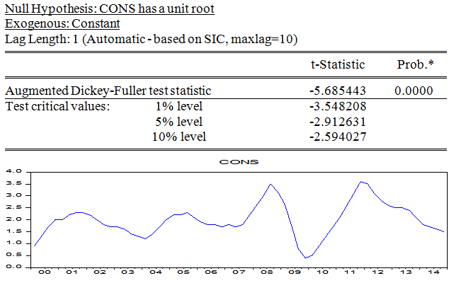
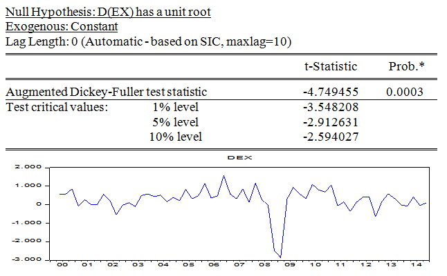
The Consumer price is stationary at p-value 0.000 which is less than 0.05 of critical value. We reject null hypothesis and accept the alternative that the consumer price is stationary.

Fig. 1 – Austria: Consumer price.

Source: prepared by the author. Used: Eviews.

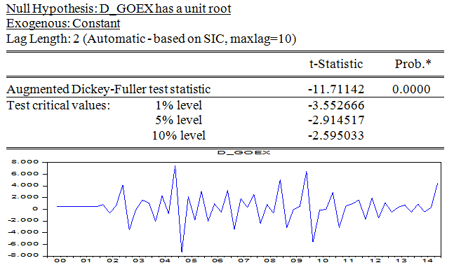
The Government spending is stationary at first differencing at 0.000 which is less than 0.05 of critical value. We reject null hypothesis and accept the alternative that the Government expenditure is stationary.

Fig. 2 – Austria: Government spending.

Source: prepared by the author. Used: Eviews.

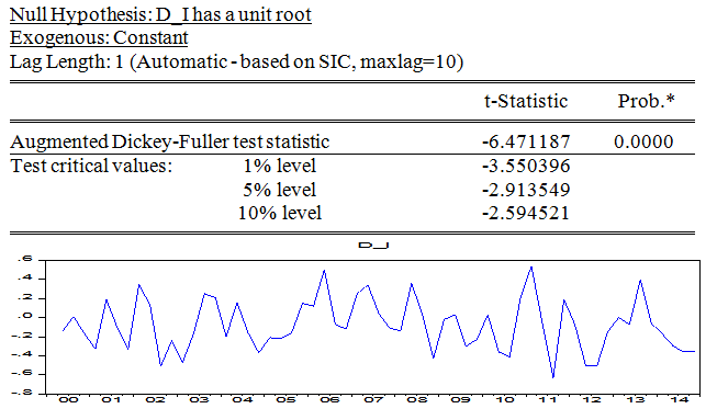
The Interest rate is stationary at first differencing at 0.000 which is less than 0.05 of critical value. We reject null hypothesis and accept the alternative that the interest rate is stationary.

Fig. 3 – Austria: Interest rate.

Source: prepared by the author. Used: Eviews.

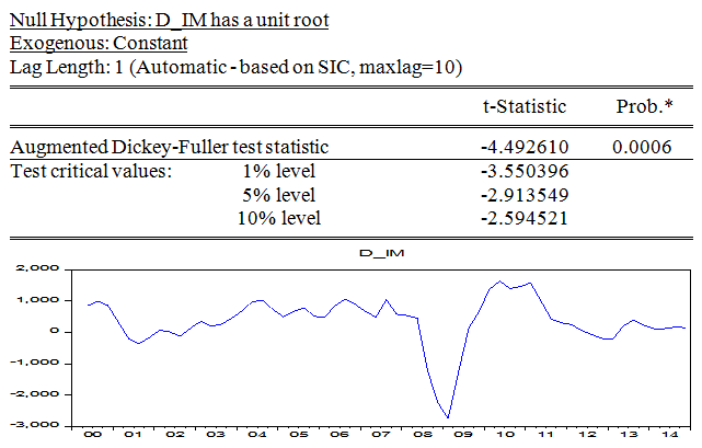
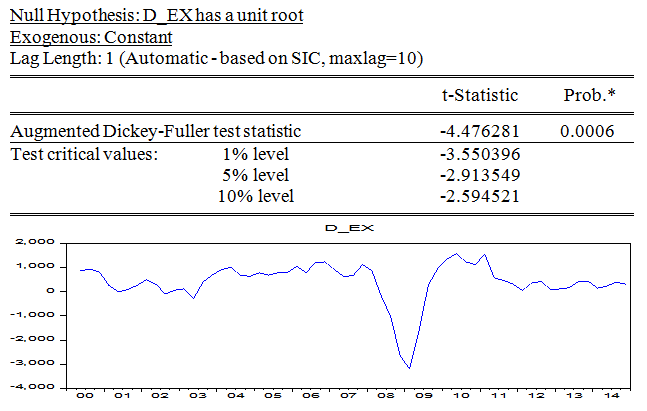
The Import is stationary at first differencing at 0.0006 which is less than 0.05 of critical value. We reject null hypothesis and accept the alternative that the import is stationary.

Fig. 4 – Austria: Import.

Source: prepared by the author. Used: Eviews.

The Export is stationary at first differencing at 0.006 which is less than 0.05 of critical value. We reject null hypothesis and accept the alternative that the export is stationary.

Fig. 5 – Austria: Export.

Source: prepared by the author. Used: Eviews.

 

Lithuania Data

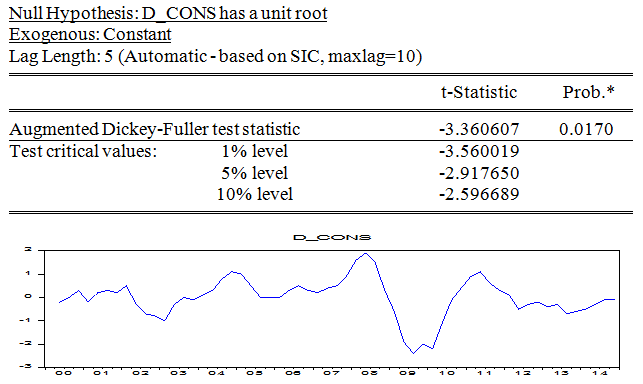
The Consumer price is stationary at first differencing at 0.0170 which is less than 0.05 of critical value. We reject null hypothesis and accept the alternative that the consumer price is stationary.

Fig. 6 – Lithuania: Consumer price.

Source: prepared by the author. Used: Eviews.

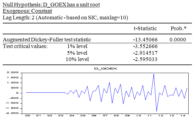
The Government spending is stationary at first differencing at 0.0000 which is less than 0.05 of critical value. We reject null hypothesis and accept the alternative that the government expenditure is stationary.

Fig. 7 – Lithuania: Government spending.

Source: prepared by the author. Used: Eviews.

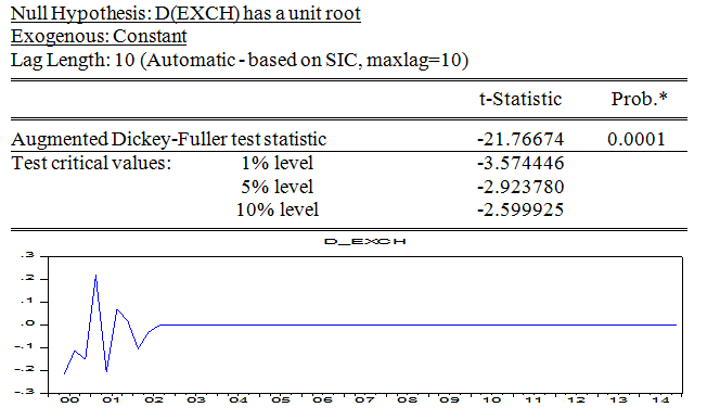
The Exchange rate is stationary at first differencing at 0.0001 which is less than 0.05 of critical value. We reject null hypothesis and accept the alternative that the exchange rate is stationary.

Fig. 8 – Lithuania: Exchange rate.

Source: prepared by the author. Used: Eviews.

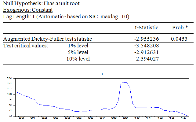
The Interest rate is stationary at 0.0453 which is less than 0.05 of critical value. We reject null hypothesis and accept the alternative that the interest rate is stationary.

Fig. 9 – Lithuania: Interest rate.

Source: prepared by the author. Used: Eviews.

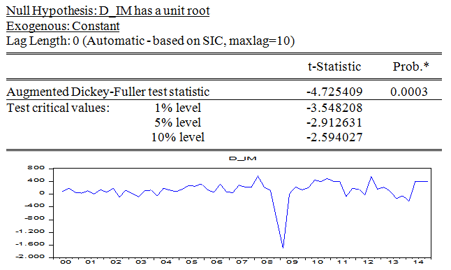
The Import is stationary at first differencing at 0.0003 which is less than 0.05 of critical value. We reject null hypothesis and accept the alternative that import is stationary.

Fig. 10 – Lithuania: Import.

Source: prepared by the author. Used: Eviews.

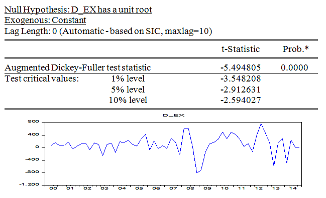
The Export is stationary at first differencing at 0.000 which is less than 0.05 of critical value. We reject null hypothesis and accept the alternative that the export is stationary.

Fig. 11 – Lithuania: Export.

Source: prepared by the author. Used: Eviews.

 

Kazakhstan data

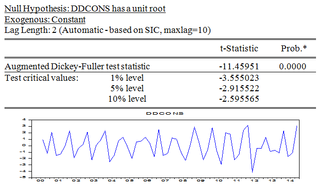
The Consumer price is stationary at second difference at p-value of 0.000 which less than critical value of 0.05. We reject the hypothesis and accept the alternative that consumer price is stationary.

Fig. 12 – Kazakhstan: Consumer price.

Source: prepared by the author. Used: Eviews.

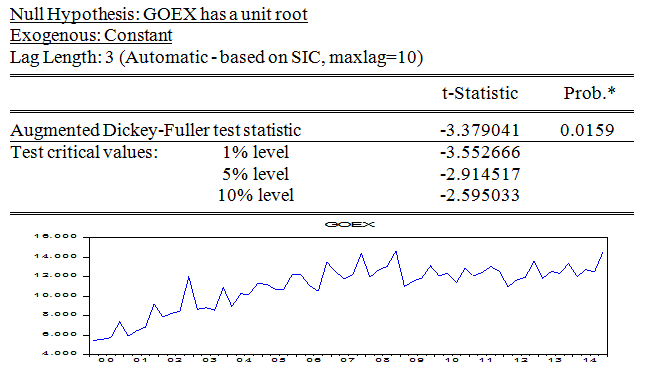
Government Spending  is stationary at 0.0159 which is less than 0.05 critical value. We reject the hypothesis and accept the alternative that, government spending is stationary.

Fig. 13 – Kazakhstan: Government spending.

Source: prepared by the author. Used: Eviews.

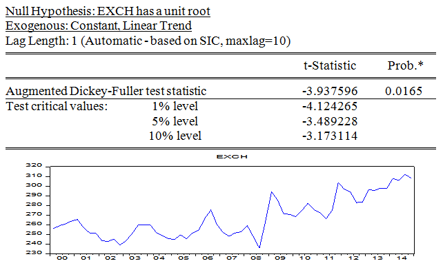
Exchange rate is stationary with intercept and trend at 0.0165 which is less than 0.05 critical value. We reject the hypothesis and accept the alternative that, exchange is stationary.

Fig. 14 – Kazakhstan: Exchange rate.

Source: prepared by the author. Used: Eviews.

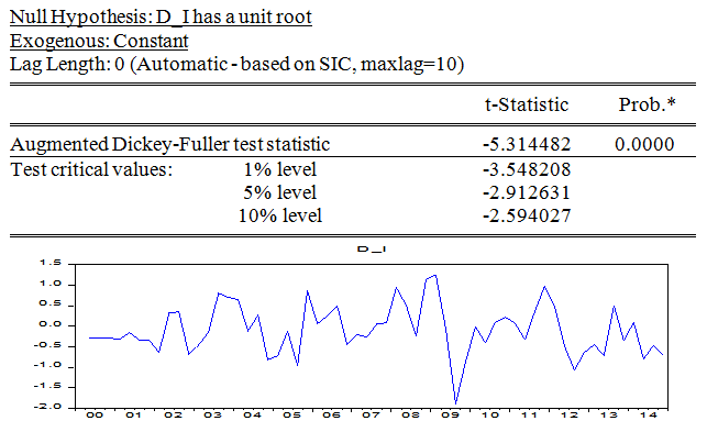
Interest rate is stationary at first differences at p-value 0.000 which is less than 0.05 of the critical value; we therefore reject the null hypothesis and accept the alternative that interest rate is stationary.

Fig. 15 – Kazakhstan: Interest rate.

Source: prepared by the author. Used: Eviews.

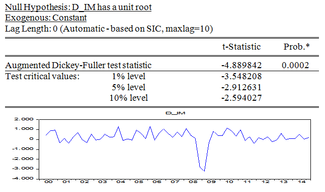
The Import is stationary at first differences at p-value 0.0002 which is less than 0.05 of the critical value. We therefore reject the null hypothesis and accept the alternative the import is stationary.

Fig. 16 – Kazakhstan: Import.

Source: prepared by the author. Used: Eviews.

The Export is stationary at first differences at p-value 0.0003 which is less than 0.05 of the critical value; we therefore reject the null hypothesis and accept the alternative the export is stationary.

Fig. 17 – Kazakhstan: Export.

Source: prepared by the author. Used: Eviews.

 

Analysis

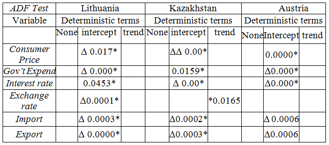
Lithuania and Kazakhstan share some similar patterns, among them is Consumer price which  have to be differenced once for Lithuania and twice for Kazakhstan to be stationary while for Austria it is already stationary. The goverenment spending of Lithuania and Austria are stationary at first difference while that of Kazakhstan is stationary with intercept without differencing. Kazakhstan and Austria have first difference in interest rate while Lithuania tend to be statioanry without differencing. All the three countries shares first diffenceing in their import and export to be stationary (Table 1).

Table 1 – Stationarity test of variables.

∆ , ∆∆ denotes the first and second difference respectively

*   significance at p-value

Source: prepared by the author. Used: Eviews.

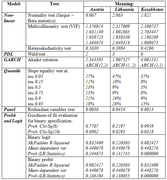
Table 2 – Model analyses (test results).

Source: prepared by the author. Used: Eviews.

The Dummy variable is dependent variable that can take on only 2 values, 0 or 1. In our case it is CRISIS that is equal to 1 from 3rd quarter 2008 till end 2012 and 0 otherwise and it shows the consequences of the financial crisis. The explanatory variables of the dummy explain highly of financial crises in Kazakhstan with R-square of 73 percent, adjusted R-square 70 percent in which constant, exchange rate and government expenditure are all significant, mostly importantly the overall model is significant at p-value of 0.000. In constrast to Lithuania and Austria in which the model explain very low of financial crises at R-square of 15 percent and 11 percent respectively and both model F-statistic are insignificant.

The Polynomial Distributed Lags (PDL) stated not reject the null hypothesis of addition lags of three (3) and beyond for Lithuania, while Kazakhstan is at eight (8) and Austria two (2).

Testing for Non-Linear models among the said countries have low R-square to explain non-linear regression, although the overall model is siginificant with one or two individual coeffiecent(s) been singificant.

The normality test of Jarque-Bera P-value was 0.067, 2.863 and 1.821 for Austria, Lithuania and Kazakhstan respectively, which are all more than 0.05 therefore, do not reject null hypothesis and stated that residuals are normal distributed.

The Variance Inflation Factors is between 1 and 3 in all the observed countries, indicates multicollinearity is low.

The test for Heteroscedasticity were 0.3984, 0.5639 and 0.4206 for Lithuania, Austria and Kazakhstan and are greater than 0.05 of critical of p-value therefore, do not reject null hypothesis and accept the alternative the residuals are Homoscedasticity, mean series should exhibit fluctuation around a constant long run mean, has a finite variance and has a theoretical correlogram (Enders W., 2003).

The Redundant variables test are conduct jointly to verify coefficients, Austria, Lithuania and Kazakhstan have 0.0036, 0.0454 and 0.0014 p-values which are less than 0.05 of critical value, therefore reject the null hypothesis and accept the alternative the coefficients are not redundant and they should not be omitted from the model.

The estimation of the best GARCH model differs slightly across the observed countries, Kazakhstan has minimum Akaike Criterion of 4.001531 at ARCH (1,1), Lithuania has minimum Alkaike criterion ARCH (1, 2) of 1.907527 while Austria has minimum at ARCH (2,2) of Alkaike criterion 1.343595, comparing the three countries the Austria has the smallest Alkaike follow by Lithuania and then Kazakhstan, see graphs below.

Fig. 18 – GARCH models.

Source: prepared by the author. Used: Eviews.

The estimation of Probit in Kazakhstan has Mc Fadden R-square of 83 percent with three  individuals coefficients significant greater than one  percent of Logit Mc Fadden R-square (82 percent) although they have the similar coefficients significant and all overall regression of Prob (LR statistic of 0.000), therefore assume that the model can predict crises in Kazakhstan. The dependent variable frequencies are 55 percent for non crises and 45 percent for crises. The goodness of Fit show mixed result as H-L statistic has higher value of 0.9959 and Andrew has 0.0318.

In the other hand, Austria and Lithuania Probit and Logit are insignificant to explain the crises. Their Mc Fadden R-square was 8.3 percent and 12.0 percent in Probit and Logit with Prob (LR statistic of 0.24 and 0.13) respectively. The dependent variable frequencies are 66 percent and 56 percent for non crises and 34 percent and 44 for crises respectively.

The Goodness of fit evaluation for binary specification have Adrews low values at 0.0293 and H-L statistic is high (0.2197) for Lithunia as mixed result while Austria has high (0.7707 and 0.6962) in both Adrews and H-L stattistic.

Some reasons the author prefers to use Quantile: analysis of the distributions rather than average, unequal variation of samples, interest in representative values, tail distributions and it’s robustness. The Quantile regression at tau 0.05, Lithuania has Pseudo R-square of 47 percent more 27 percent higher of Austria and 37 percent higher than Kazakhstan. Again at tau 0.25, Lithuania has the highest of 18 percent, Austria 11 percent and Kazakhstan lowest of 8 percent. For tau 0.5, Austria has 13 percent, Kazakhstan 9 percent and lowest is Lithuania with 5 percent. Quantile tau at 0.75, Again Austria led with 15 percent, Kazakhstan 9 percent and Lithuania has 8 percent. For tau at 0.9, Austria has 21 percent; Lithuania has 19 percent, and Kazakhstan 9 percent. And finally at tau 0.95, Lithuania has 26 percent, Austria 18 percent and Kazakhstan with the least of 15 percent.

Based on Quantile regression result, the responses of Lithuania economy to consumer price is more shifted to the poor and rich against the average people, as for Austria responses tend to more on average and rich than the poor and while Kazakhstan tend to maintain balance. The graph of the said countries reveals that coefficients differ across Quantile values and that the conditional Quantiles are identical.

Panel data, the Fixed Effect Model of the observed countries has R-square of 99 percent, while Random has R-square 96 percent with both F-statistics at 0.000 significant level of p-value. The cross section effect between the Lithuania and the two countries (Austria and Kazakhstan) is 22.21 percent. In the contrary Austria against the Kazakhstan and Lithuania is negative 16.23 and while Kazakhstan against Lithuania and Austria is also negative but 43.39 percent.

The Cross-section F” and “Cross-section Chi-square” evaluate the joint significance of the cross section effects both at p-value of 0.00 indicated that the two statistic values and the associated p-values strongly reject the null that the cross-section effects are redundant.

The cross section random is 0.00 provides much evidence against the null hypothesis that there is misspecification. The additional test detail, showing the coefficient estimates from both the random and fixed effects estimators, along with the variance of the difference and associated p-values for the hypothesis that there is similarity between the two estimate suggests that unobserved heterogeneity is not creating a large bias in the simple.

Husman test also provided additional proof of p-value at 0.000 is significant to reject null and accept the alternative that the unobserved heterogeneity is correlated with the explicators. Therefore, Fixed Effect is more consistent in this panel regression and the author prefers it.

In Austria, Lithuania and Kazakhstan the minimum error in Dummy to predict crises were 0.094, 0.140 and 0.01, in Logit forecast error was 0.107, 0.142 and 0.02 while in Probit (0.142, 0.0960 and 0.02) respectively. However, forecasting error for consumer price in Austria has equal minimum error of 0.0006 for Non-linear and GARCH against Quantile regression of 0.005 while Lithuania and Kazakhstan has its minimum error in Quantile of 12.186 and 0.00001 respectively. The total forecast errors for the Austria and Kazakhstan is small at 0.30 and 0.016 respectively.

Comparative tables of the final results of all the applied models are shown below:

Table 3 – Kazakhstan:

Source: prepared by the author. Used: Eviews.

Table 4 – Austria:

Source: prepared by the author. Used: Eviews.

Table 5 – Lithuania:

Source: prepared by the author. Used: Eviews.

 

Conclusion

The research variables are differencing variables as expected in time series data.

The conditional convergence among these countries is factor of structural differences, as Kazakhstan and more of Lithuania need to growth and Austria less to meet in convergence.

Finally, based on the result, the financial crises have more impact on Lithuania and Kazakhstan more than Austria. The best model for Lithuania is Dummy with forecast error of 0.140, Austria best model should be GARCH and Non-Linear with the same forecast error of 0.0006 and Kazakhstan best model shall be Quantile which has forecast error of 0.0001 (Tables 3, 4, 5).

In the course of the work concluded that the current trends of world development necessitate a balance between the national interests of individual countries and the interests of global development. This task is greatly complicated the unfolding global financial and economic crisis. It is not just about the protection of national interests of individual countries or regional groupings, but on the formation of such an economic model that will provide a balance between anti-crisis programs and the preservation of development potential. In addition, the formation of a new macroeconomic model and the global financial architecture, suggest the need for justification of the strategic goals of development and the development of long-term socio - economic programs, as well as an effective evaluation.

References

1. Arestis P., Demetriades P. Financial development and economic growth: Assessing the evidence. TheEconomicJournal. 1997, 107, May, р 783–799.
2. Demetriades P., Hussein K. Does Financial Development Cause Economic Growth? Time Series Evidence from Sixteen Countries.Journal of Development Economics.1996, 51 (2), р387-411.
3. Levine R., Loayza N., Beck T. Financial Intermediation and Growth: Causality and Causes. Journal of Monetary Economics. 2000, 46, pp. 31-77.
4. Lynch D. Measuring financial sector development: A study of selected Asia-Pacific countries. The Developing Economies. 1996, 34, March, pp. 3–33.
5. Stiglitz J. Financial Systems for Eastern Europes Emerging Democracies. ICS press, San Francisco, Cal., US, 1993, pp. 9-10.
6. Demetriades P., and S. Andrianova. Finance and growth: what we know and what we need to know. University of Leicester. October 19, 2003. 25 p.
7. Demirguc-Kunt, A. and E. Detragiache. Financial Liberalization and Financial Fragility/ B. Pleskovic and J. Stiglitz, eds., Annual World Bank Conference on Development Economics 1998, Washington DC: World Bank: Reuters, Pearson Education, 1999, pp. 303–331.
8. Kaminsky, G. L. and C. M. Reinhart. The Twin Crises: the Causes of Banking and Balance-of-Payments Problems// American Economic Reviews, 1999, 89 (3), pp. 473–500.
9. King, R. G. and R. Levine. Finance and Growth: Schumpeter Might be Right// Quarterly Journal of Economics, 1993, 108, 717–737.
10. La Porta, R., F. Lopez-de-Silanes, A. Shleifer, and R. Vishny. Government Ownership of Banks// Journal of Finance, 2002, 57(1), pp. 265–301.
11. Rajan, R. and L. Zingales. The Great Reversals: The Politics of Financial Development in the 20th Century// Journal of Financial Economics, forthcoming 69, 2003, 5-50.
12. Keynes, John M.The General Theory of Employment // The Quarterly Journal of Economics. — 1937.
13. Global Financial Stability Report. Iss. 2004–2012. IMF, Washington.
14. Akerlof G., Shiller R. Animal Spirits, etc. Princeton: Princeton University Press, 2009.
15. Krugman P. End This Depression Now! L.: W.W. Norton, 2012.
16. Stiglitz J. Needed: A New Economic Paradigm // Financial Times. 2010. August 20.
17. Ghosh A., Ostry J., Tamirisa N. Anticipating the Next Crisis // Finance and Development. September 2009. Washington.
18. Encyclopedia of Complexity and Systems Science. Berlin/Hеidelberg: Springer, 2009.
19. Stanley H.E., Gopikrishnan P., Plerou V., Salinger M.A. Patterns and Correlations in Economic Phenomena Uncovered Using Concepts of Statistical Physics // Lecture Notes in Physics (Series). Vol. 621. Berlin/Heidelberg: Springer, 2003.
20. Newman M.J.E. Power Laws, Pareto Distributions and Zipf’s Law. 2006. (arXiv: cond-math/0412004 v3 29 May 2006)
21. Vasicek O. Probability of Loss on a Loan Portfolio: Working Paper, KMV Corporation. San Francisco, 1987.
22. Smirnov A. Finansovyi rychag i nestabilnost // Voprosy krizisa. 2012. № 9.
23. Adrian T., Shin H. Liquidity and Financial Contagion, Banque de France // Financial Stability Reviews. 2008. № 11.
24. Farmer D. Market Force, Ecology and Evolution. Santa Fe: Santa Fe Institute, 2000.
25. Knight F. Risk, Uncertainty and Profit. Washington: Beard Books, 2002.
26. Dimitrios, A. Applied Econometrics, A modern approach using Eviews and microfit, 2006.
27. Enders, W. Applied Econometric Time Series, second edition. Wiley, 2003.
28. Greene, W.H. Econometric Analysis, 5^th edition, 1993.
29. Euro area statistics: https://www.euro-area-statistics.org
30. The official website of the Financial supervision of the National Bank of the Republic of Kazakhstan: http://www.afn.kz/
31. The official website of the Agency on statistics of the Republic of Kazakhstan: http://www.stat.kz/Pages/default.aspx.
32. The official website of the National Bank of the Republic of Kazakhstan: http://www.nationalbank.kz/.
33. Statistical Bulletin of the National Bank of the Republic of Kazakhstan: http://www.nationalbank.kz/index.cfm?uid=ED7C51EE-2219-B830-8A138816A7576BA8&docid=310.