ДЕФОРМАЦИЯ ПОВЕРХНОСТИ ПРИ ГЕОМЕТРИЧЕСКИХ ОГРАНИЧЕНИЯХ

Берзин Д.В.

Кандидат физико-математических наук, доцент, Финансовый университет при Правительстве Российской Федерации, Москва

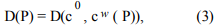
ДЕФОРМАЦИЯ ПОВЕРХНОСТИ ПРИ ГЕОМЕТРИЧЕСКИХ ОГРАНИЧЕНИЯХ

Аннотация

Предположим, что мы хотим изменить (деформировать) NURBS минимальным образом, чтобы достичь условия непрерывности с ее соседями. В данной работе дается алгоритм такой деформации

Ключевые слова: система автоматизированного проектирования, условие непрерывности G,  NURBS, вариационная задача.

Berzin D.V.

PhD,  Associate Professor, Financial University under the Government of the Russian Federation, Moscow

SURFACE DEFORMATION WITH GEOMETRIC CONSTRAINTS

Abstract

Suppose we want to deform a base surface of a face in order to achieve some continuity condition (e.g., G continuity) with the given neighbors at common edges. We give an algorithm of a deformation that changes the surface geometry as little as possible.

Keywords: CAD, G¹ continuity, NURBS, variational problem.

Suppose that a face F0 is surrounded by some number of neighbor faces F1, F2, … . We want to deform an (initial) base surface of F0 in order to achieve some continuity condition (e.g., G¹ continuity) with the given neighbors at common edges. This deformation should change the surface geometry as little as possible.

1. “Curve error” functional

Denote vectors of initial and deformed control points by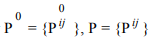respectively.　Consider a curve , which belongs to (or located near) the initial (not deformed) surface  Let

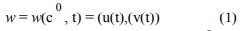
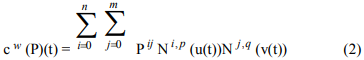
be a corresponding uv-curve of c(t). Consider a class of 3D-curves with a fixed w and the variable P:

Consider a functional

which in some way expresses distance (or maximum gap) between initial and deformed curves. Let call such a functional “curve error” functional.

2. Other functionals

Consider two more types of functionals: H(P) and G(P). “Control point error” functional H(P) expresses a distance between sets of control points P and P. H(P) is to control a deviation of a deformed surface. “Continuity error” functional G(P) is to keep some continuity condition, for example, G¹ with some of neighbor faces.

3. Quasi-G¹

Instead of G¹ at sample points on boundary curves, we can try to achieve a little different (and, in some meaning, stronger, than G¹) condition, which, however, leads to linearity in the variational problem. Let E be an arbitrary, but fixed sample point on some edge, which is shared by both face F0 and the neighbor face F1. Consider   a tangent plane  at E to a base surface of the face F1. Let and be corresponding tangent vectors (taken at the point E in u and v directions respectively) to the initial base surface S(P⁰) of the F0. Project and onto , get the pair of vectors  and  respectively. Now we can compose the continuity error functional for this condition at the point E:

where and  - corresponding tangent vectors to the deformed surface S(P), and  and  are real variables. Respectively, continuity error functional for a set of sample points

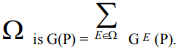
4. Variational problem

Now, we can compose the “total error” functional

where constants can serve as weights and might be found empirically. Eventually, our goal is to find a minimum:

This variational problem without restrictions (see [4]) can be solved according to the Fermat theorem:

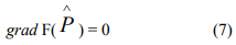
where  is a solution of the problem.

5. Remarks

In this approach, knot vectors and the number of control points are still the same after deformation. Perhaps, this restriction will not allow achieving a precise continuity condition and preserving boundary curves within prescribed tolerances. It is needed to measure continuity and curve errors, and, if necessary, insert additional knots in the initial surface, and after that restart the deformation.

All terms in (5) should have a quadratic form, so that the system (7) becomes linear. In our first implementation, we will assume for simplicity.

Quasi-G¹ condition is not the same as G¹, but we can expect that generally (6) will force the corresponding tangent planes to approach desired positions. 

6. First example

Let’s consider a simple example of variational problem with geometric constraints. Suppose that point A is located inside a mimimax box of points C and D. It is needed to find a new position B of the point A, so that B is nearly equidistant from both C and D (i.e. |BC-BD| -> min) and the movement (deformation) is mimimal (i.e. |AB| -> min). Obviously, it’s reduced to a problem with one coordinate, say x. If x⁰ stands for A, x¹ - for C, x² - for D, and – for unknown B, then minimization of corresponding functional leads to

7. Second example

To exemplify, how to find a minimum of functionals like (4), consider another simple variational problem with geometric constrains. Find a point (x,y), which is as close as possible to both line (0,2) and the point (2,1). To solve this problem, compose the functional

and find its minimum. Equation

grad F(x, y, ) = 0

leads to the following expressions:

4x - 4 = 0,  4y - 4 - 2 = 0,  -4y + 8 = 0

The answer: = 0.5 and the point is (1,1).

8. Expressions for the curve error functional

After discussing the general approach, we are ready to write out precise expressions for the curve error functional D(P). Consider an arbitrary, but fixed pair w = (u,v), and corresponding 3D point E = E(P, w) on a loop of F0. Then, according to (2),

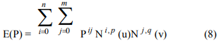
Set 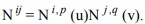. Renumber (i,j) -> k and rewrite the expression (8) as

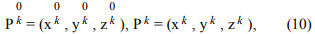
where N = (n+1)(m+1)-1, i.e. N is the total number of control points in the control net. Suppose that for deformed surface control points have the following coordinate representation:

where k = 0,…,N.

Then the squared movement of a sample point with fixed uv-coordinates w is

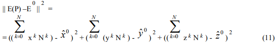
Here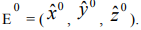

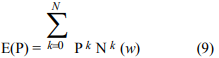
If the total number of sample points (to control the curve movement) on the curve(s) is d+1, then the functional D(P) takes the form

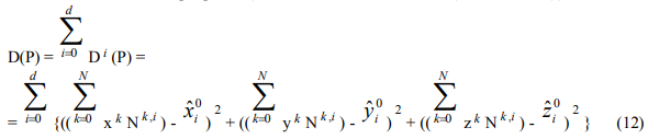
where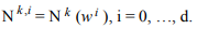

Corresponding partial derivatives of D(P) with respect to the variables are

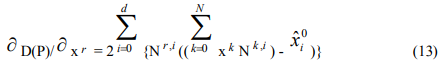
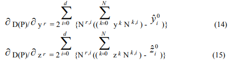
where r = 0, …, N.

1. Expressions for the control point error functional

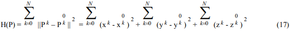
The squared movement of a k-th control point is

The control point error functional

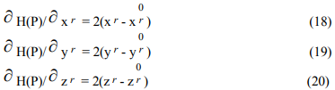
Corresponding partial derivatives of H(P) with respect to the variables are

2. Expressions for continuity error functional

Consider again an arbitrary, but fixed pair w = (u,v), and corresponding 3D point E = E(P, w) on a loop of the F0. Then tangent vectors to the surface S(P) at this point:

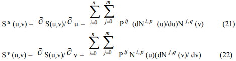
Denote . Renumber (i,j) -> k, then we rewrite expressions (21) and  (22) as

    

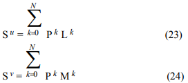
where N = (n+1)(m+1)-1. Suppose, that 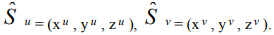 Then the expression (4) takes the form:

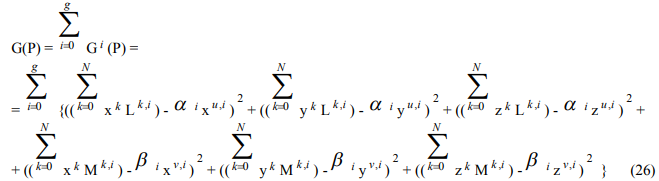
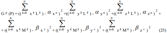
Suppose now, that the total number of sample points E (to control the continuity) on the curve(s) is g+1. Denote corresponding projections of tangent vectors by and corresponding coefficients byand respectively, and 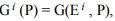, where i = 0, … , g. Then the functional G(P) takes the form

Corresponding partial derivatives of G(P) with respect to the variables 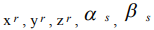 are

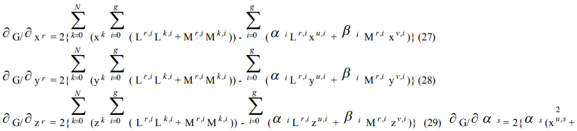
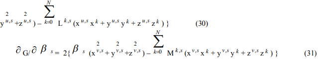
where r = 0, …, N and s = 0, …, g.

1. 　Linear system for the variational problem

We want to solve the variational problem (6). Actually, in our task the functional is a functional of 3(N+1)+2(g+1) variables. Namely, we have (N+1) unknown control points of the deformed surface (3 coordinates each), and (g+1) variable for each of u and v direction in the continuity keeping component. Now we are ready to write out precise expressions for (5). For simplicity, set

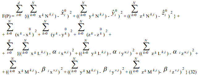
The system (7) takes the form:

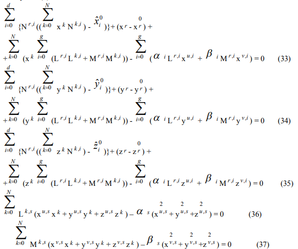
The system (33)-(37) is a linear system of 3(N+1)+2(g+1) equations and 3(N+1)+2(g+1) unknowns. Here r = 0,…, N and s = 0,…, g. Denote:

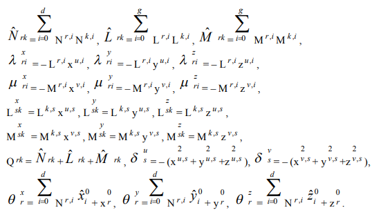
Then we get the following expressions:

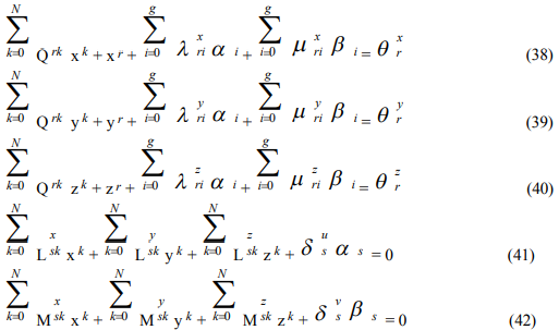
Solution of the (38-42) is the solution of the problem. This linear system has the form

AX = B                                                                    (43)

where A = (a ^ij) is a matrix of constants, B = (bⁱ) is a vector of constants, and i, j = 0, …, 3(N+1)+2(g+1) – 1. The vector of unknowns is

We can depict the structure of (43) in the following sketchy form (see the next chapter for a full description):

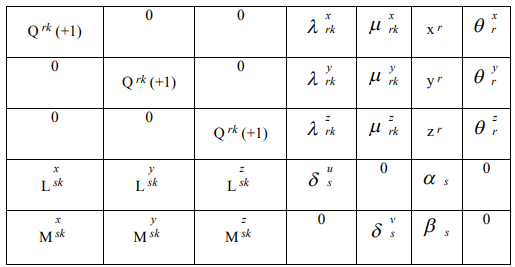
1.  The matrix

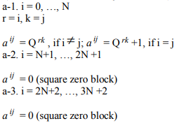
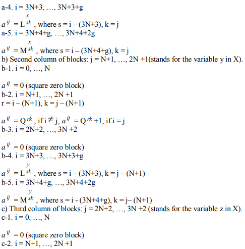
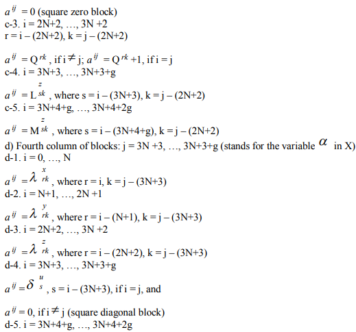
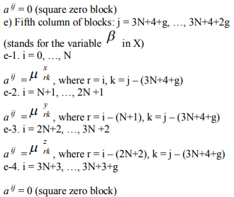
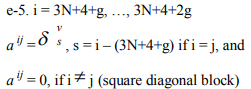
The matrix A in (43) consists of 25 blocks and can be described as follows.

a) First column of blocks: j = 0, …, N (stands for the variable x in X).

14. Algorithm

In order to compute new positions of control points, we should complete the following main steps:

1) Get a vector of (N+1) control points of initial surface, see (10).

2) Choose (d+1) sample points to keep boundary curve(s) position 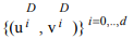. Let’s call these points “G0 sample points”.

3) Choose (g+1) sample points to keep continuity 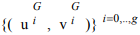. Let’s call these points “G1 sample points”. In our implementation, a set of G1 sample points is a subset of the set of G0 sample points. 　　　

4) Calculate “desired” tangent plane at each G1 sample point and get 2(g+1) corresponding projections of tangent vectors to initial surface onto the tangent plane: () and (), see (26). In other words, get a pair of 3D vectors for each G1 sample point.

5) Calculate two vectors of (g+1) constants each:

6) Calculate (N+1)-vector N^{k ,i} for each G0 sample point using B-spline basic functions, see (12).

7) Calculate a pair of (N+1)-vectors (L^{k ,i}), (M^{k ,i}) for each G1 sample point using B-spline basic functions and their derivatives, see (26).

8) Calculate three (N+1)(N+1) matrices: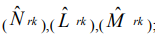; see Ch.11.

9) Calculate (N+1)(N+1) matrix (Q^rk), see Ch.11.

10) We don’t need matrices () and () anymore and can free corresponding memory.

11) Calculate 3 vectors of (N+1) constants each: 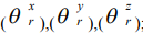; see Ch.11.

12) We don’t need the matrix () and vector of control points anymore and can free corresponding memory.

13) Calculate six (N+1)(g+1) matrices 

14) Calculate six (g+1)(N+1) matrices

15) Free memory allocated for each sample point.

16) Compose the matrix A. Free corresponding memory.

17) Compose right-side array of constants B.

18) Solve the system (43) using routines for sparse linear equations.

19) Get a set of new control points.

20) Create new surface.