ПОСТАНОВКА КРАЕВОЙ ЗАДАЧИ НА ГРАФЕ
ПОСТАНОВКА КРАЕВОЙ ЗАДАЧИ НА ГРАФЕ
Научная статья
Шаждекеева Н.К.1, *, Жакатай Е.С.2
1, 2Атырауский государственный университет имени Х.Досмухамедова, Атырау, Казахстан
* Корреспондирующий автор (n.shazhdekeeva[at]mail.ru)
АннотацияДифференциальные уравнения, встречающиеся в разных приложениях, могут быть интерпретированы как уравнения в графах. Есть веские основания утверждать, что теория таких уравнений может применяться в широких масштабах, и свойства графа могут быть использованы для создания качественной теории таких уравнений и методов их решения. Используя простые свойства графов, мы можем изучить действие решений дифференциальных уравнений. Есть основания полагать, что структура графа влияет на некоторые важные свойства решения.
Ключевые слова: граф, подграф, дифференциальное уравнение, краевая производная, краевая задача.
STATEMENT OF THE BOUNDARY VALUE PROBLEM ON THE GRAPH
Research article
Shazhedekeeva N.K.1, *, Zhakatay Y.S.2
1, 2 Atyrau State University named after Kh.Dosmukhamedov, Atyrau, Kazakhstan
* Corresponding author (n.shazhdekeeva[at]mail.ru)
AbstractDifferential equations found in different applications, can be interpreted as equations in graphs. There is good reason to argue that the theory of such equations can be applied on a large scale, and on the other hand, the properties of the graph can be used to create a qualitative theory of such equations and methods for solving them. Using the simple properties of graphs, we can study the action of solutions of differential equations. There is reason to believe that the structure of the graph affects some important properties of the solution.
Keywords: graph, subgraph, differential equation, boundary derivative, boundary value problem.
Introduction An ordinary differential equation on a segmentis the basic concept in the analysis of models of the most diverse problems of natural science. By associating such a system in the form of a spatial network (geometric graph), the researcher obtains an equation of the form (1) on each edge of such a network, and at the network nodes the interaction conditions are of the form
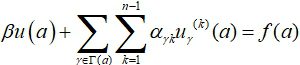
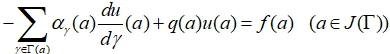
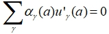 where the summation is carried out over the y edges adjacent to the a node. And at the boundary nodes, conditions of the type
Graph theory, their structure, properties and applications are studied in [1] - [5]. And differential equations on graphs are considered in [6] - [7]. In this paper, differential equations and the statement of a boundary value problem on a graph are presented.
geometric graph means a one-dimensional stratified manifold. An edge of a graph is a one-dimensional smooth regular manifold (curve). A vertex of a graph is a point. An edge is denoted by y or if they are numbered by index i, then by y1. And vertices are denoted by a (or aj). A graph is denoted by Г.
Vertex index is the number of edges adjacent to it, taking into account the multiplicity. Г(a) denotes the set of edges adjacent to the vertex a. When setting boundary value problems, the following property is useful: the sum of the indices of all vertices of the graph is equal to twice the number of edges.
Scalar function u(x) on the graph is an usual mapping as ![]() . The restriction of function u(x) to edge γ is denoted by
. The restriction of function u(x) to edge γ is denoted by ![]() .
.
The set of continuous functions on Г is denoted by С[Г]. The set of piecewise continuous functions (continuity on the edges, but the limits at the same vertex for different edges are different, no value is assigned to the function at the vertex) is denoted by С(Г) or by ![]() is understood as a disconnected formal union of edges). The set of discretely continuous (continuity on each edge as on an interval, the presence of values at the vertices, however, there is no relationship between the values at the vertices and the limits along the edges adjacent to these vertices) are denoted by
is understood as a disconnected formal union of edges). The set of discretely continuous (continuity on each edge as on an interval, the presence of values at the vertices, however, there is no relationship between the values at the vertices and the limits along the edges adjacent to these vertices) are denoted by ![]() .
.
![]() denotes the space of functions on each edge times continuously differentiable up to the boundary (i.e., all derivatives belong to С[Г]). The differential operator is defined in this space. In order not to write separately the continuity conditions at the vertices of the graph, it is convenient to pose the problem in space
denotes the space of functions on each edge times continuously differentiable up to the boundary (i.e., all derivatives belong to С[Г]). The differential operator is defined in this space. In order not to write separately the continuity conditions at the vertices of the graph, it is convenient to pose the problem in space ![]() .
.
For the function from ![]() the extreme derivatives of this function
the extreme derivatives of this function
![]()
at the vertex a of the graph in the direction "inward" of the edge ![]() are introduced, here k is derivative order. These are the usual derivatives of function
are introduced, here k is derivative order. These are the usual derivatives of function ![]() given by edge γ, calculated at the endpoint (where one-way differentiation is applied).
given by edge γ, calculated at the endpoint (where one-way differentiation is applied).
A linear differential equation on an edge is an ordinary differential equation on a curve. For some fixed parameterization ![]() , it is described by the equation
, it is described by the equation
![]() (1)
(1)
and when changing the parameterization, the coefficients are recalculated according to the corresponding formulas.
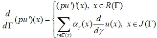
A matching condition at a vertex is any combination of the values of a function and its boundary derivatives at that vertex. Formally, this is written as
 (2)
The left-hand side of this equality is conveniently denoted by
(2)
The left-hand side of this equality is conveniently denoted by An ordinary linear differential equation on a graph Г in ![]()
![]() (3)
(3)
is any combination of linear differential equations (3) on the edges and regular matching conditions (4) at the vertices of the graph.
The set of vertices at which the Dirichlet condition is given is called the boundary of the graph and is denoted by ![]() . The vertices of a graph that are not boundary are called internal vertices.
. The vertices of a graph that are not boundary are called internal vertices.
If the edges of the graph can be smoothly parameterized and they do not intersect, then we can consider them as straight intervals. Thus we can say that the graph Г consists of non-intersecting intervals:
![]() (4)
(4)
The set of ends of the intervals is denoted by ![]() , each point from it is called the internal vertex (node) of the graph. The ends of the intervals (4), not included in
, each point from it is called the internal vertex (node) of the graph. The ends of the intervals (4), not included in ![]() , are called the boundary vertices of Г; their set is denoted by
, are called the boundary vertices of Г; their set is denoted by ![]() .
.
Any connected open subset of Г is called a subgraph. Any internal vertex of a subgraph ![]() is internal also for Г. But the set
is internal also for Г. But the set ![]() may contain points that are not included in either
may contain points that are not included in either ![]() .
.
The homogeneous differential equation in the graph looks like this:
![]() (5)
(5)
 (6)
(6)
and ![]() numbers
numbers ![]() are supposed to be positive. Solutions (5) are sought only among of functions given on all Г, and for which
are supposed to be positive. Solutions (5) are sought only among of functions given on all Г, and for which ![]() . A set of such functions are denoted by
. A set of such functions are denoted by ![]() .
.
In mathematical works, problems on networks appeared in the form of a question about continuous solutions of the system
![]() (7)
(7)
 (8)
(8)
![]() (9)
(9)
where (7) are ordinary differential equations given separately on edges ![]() , (8) and (9) are linear relationships defined locally in a finite number of points - at internal and boundary vertices of the graph Г. Basically, we consider this system as a boundary value problem
, (8) and (9) are linear relationships defined locally in a finite number of points - at internal and boundary vertices of the graph Г. Basically, we consider this system as a boundary value problem
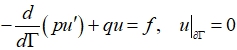 (10)
(10)
relating equalities (9) to boundary conditions, and (7), (8) to realizations on ![]() of a single equation on a whole connected set Г. Such a view, paving the way for qualitative results, leaves aside such important and traditional for ODE questions as the solvability of our ordinary differential equation on the whole of , the expendability of solutions, the dimension of the equality of solutions, etc. Answers to such questions are possible on the basis of the general theory of boundary value problems if we look at system (7) - (9) differently.
of a single equation on a whole connected set Г. Such a view, paving the way for qualitative results, leaves aside such important and traditional for ODE questions as the solvability of our ordinary differential equation on the whole of , the expendability of solutions, the dimension of the equality of solutions, etc. Answers to such questions are possible on the basis of the general theory of boundary value problems if we look at system (7) - (9) differently.
Equations (7) are quite simple, but their solutions have different arguments. This does not allow us to consider system (7) as a single equation for a vector function of a scalar argument.
If we look at system (7) as a set of equations that are not related to each other, then we must remember the condition for the continuity of solutions at internal nodes
![]()
The solvability of problem (7) - (9) on a whole or  will be determined by the interaction of all the individual connections of this problem.
Conclusion
Boundary value problems on graphs can be considered as problems on intervals. But here, special attention is paid to the inner and boundary vertices of the graph. At these vertices additional conditions are imposed on the continuity of the solutions of the boundary value problem. Reducing the problem to a standard one in order to use the results of the general theory of boundary value problems, can be carried out using one of the following methods; each method gives its appropriate version of the problem.
Decomposition method. System (7) is considered as a single equation in ![]() . Conditions (8)–(9) are generated by a system of linear and continuous functionals in
. Conditions (8)–(9) are generated by a system of linear and continuous functionals in ![]() which are defined with the participation of the incident matrix.
which are defined with the participation of the incident matrix.
Scalarizing method. The problem is reduced to one scalar equation on a segment. Each of the equations of system (5) turns into an equation on the interval, but it is violated at the ends of the interval. Conditions (8) - (9) turn into multipoint boundary conditions of nonlocal type - they connect the values and derivatives of solutions at different points.
Vector approach. The problem reduces to a standard statement in the class of vector functions. On each edge, a canonical parameterization is introduced by the segment [0, 1], after which all equations can be considered given on the segment [0], [1], and solutions on different edges turn out to be the coordinates of one vector function.
The above methods are useful when using individual results of the classical theory.
| Конфликт интересов Не указан. | Conflict of Interest None declared. |
Список литературы / References
- Оре О. Теория графов / Оре О. – М.: Наука. Гл. ред. физ.-мат. лит., 1980. – 336с.
- Берж К. Теория графов и ее применение / Берж К. - М.: Изд-во иностр. лит., 1962. — 320 с.
- Шаждекеева Н.К. Графтар теориясындағы есептердің дифференциалдау әдісі / Шаждекеева Н.К., Айғабыл М., Батырханов А.Г. // IV Международная научно-практическая конференция «Европа и тюркский мир: наука, техника и технологии» г. Стамбуле (Турция) 1-3 мая 2019 г. 283 стр
- Шамишева А.С. Дифференциалдық теңдеулердің графтар арқылы кескіні / Шамишева А.С., Шаждекеева Н.Қ. // Білім – Ғылым - Қоғам: Өзараықпалдастық мәселелері мен перспективалары атты Халықаралық ғылыми- практикалық конференциясының материалдары, 1-бөлім. – 2013 ж. – 531-534 б.
- Шамишева А.С. Графтарды дифференциалдау / Шамишева А.С., Шаждекеева Н.Қ. // «Бектаев оқулары-1: ақпараттандыру – Қоғам дамуының болашағы» атты Халықаралық ғылыми-тәжірибелік конференциясының материалдары, 2-бөлім. – 2014 ж. – 335-340 б.
- Жапсарбаева Л.К. Самосопряженные сужения максимального оператора на графе. / Жапсарбаева Л.К., Кангужин Б.Е., Коныркулжаева М.Н. // Уфимский математический журнал. Том 9. № 4 (2017). С. 36-44.
- Покорный Ю.В. Дифференциальные уравнения на геометрических графах / Покорный Ю.В., Пенкин О.М., Приядиев В.Л. и др. М.:ФИЗМАТЛИТ. 2005. – 272 с.
Список литературы на английском языке / References in English
- Ore O. Teoriya grafov [Graph theory] / Ore O. – M.: Science. Ch. ed. Phys.-Math. lit., 1980. – 336 p. [in Russian]
- Berge K. Teoriya grafov i yeye primeneniye [Graph theory and its application] / Berge K. – M.: Publishing house of foreign countries. lit., 1962. – 320 p. [in Russian]
- Shazhdekeeva N.K. Graftar teorïyasındağı esepterdiñ dïfferencïaldaw ädisi [Methods of differential calculus in graph theory] / Shazhdekeeva N.K., Aigabyl M., Batyrkhanov A.G. // IV Mejdwnarodnaya nawçno-praktïçeskaya konferencïya «Evropa ï tyurkskïy mïr: nawka, texnïka ï texnologïï» [IV International scientific-practical conference "Europe and the Turkic world: science, technology and technology"] // Istanbul (Turkey) 1-3 May 2019 g. Page 283 [in Kazakh]
- Shamisheva A.S. Dïfferencïaldıq teñdewlerdiñ graftar arqılı keskin [Graphic representation of differential equations by graph] / Shamisheva A.S., Shazhekeeva N.K. // [EducatioN - Science - Society: Proceedings of the International Research and Practice Conference, Parts and prospects]. – 2013 – p. 531-534 [in Kazakh]
- Shamisheva A.S. Graftardi dïfferencïaldaw [Graphic differentialization] // «Bektaev oqwlari-1: aqparattandirw – qoğam damwiniñ bolaşaği» attı Xalıqaralıq ğılımï-täjirïbelik konferencïyasınıñ materïaldarı [Proceedings of the International Scientific and Practical Conference "Bektaev Readings-1: information - future of social development"] / Shamisheva A.S., Shazhekeeva N.K. part 2. – 2014 – P. 335-340 [in Kazakh]
- Zhapsarbaeva L.K. Samosopryazhennyye suzheniya maksimal'nogo operatora na grafe [Self-adjoint restrictions of maximal operator on graph] / Zhapsarbaeva L.K., Kanguzhin B.E., Konyrkulzhaeva M.N. // Ufimskiy matematicheskiy zhurnal [Ufa Mathematical Journal]. Volume 9. – 4 (2017). – P. 36-44. [in Russian]
- Pokorny Yu.V. Differentsial'nyye uravneniya na geometricheskikh grafakh. [Differential equations on geometric graphs] / Pokorny Yu.V., Penkin O. M., Priyadiev V. L. et al. // : Physmatlitis. 2005. – 272 p. [in Russian]